By Warren D. Smith. Email comments to: warren.wds AT gmail.com.
Draft#1: 20 June 2008. Draft#2: 31 July 2008. Draft#3: 21 August 2008. Draft#4 (essentially final): 25 Sept. 2008. Draft#5: 26 Sept. Declaring it final 27 January 2009.
I contend the only correct objective mathematical way to measure the "quality" of a voting system is "Bayesian Regret" (BR). Contrary to common mythology about Arrow's Impossibility Theorem, "best" voting systems can exist under this metric. This paper
Ken Arrow's impossibility theorem (1956) misled political science into a bad direction for half a century. It is commonly claimed that Arrow "showed that no 'best' voting system could exist" and then genuflections are made toward Arrow's Nobel Prize in Economics and the matter is considered closed.
Example: Paul Samuelson wrote in 1972: "What Kenneth Arrow proved once and for all is that there cannot possibly be found such an ideal voting scheme: The search of the great minds of recorded history for the perfect democracy; it turns out, is the search for a chimera, for a logical self-contradiction."But this claim is false. Arrow actually showed that single-winner voting systems based on rank-order ballots must have at least one of three bad-seeming properties. He showed nothing about voting systems not based on rank-order ballots. Also, Bayesian statistics offers a framework ("Bayesian Regret" BR) within which the "goodness" of any single-winner voting system can be objectively defined and measured to arbitrary accuracy, and in which best voting systems can exist.
This quote is simply invalid because as worded it refers to all voting schemes, not just the subclass Arrow's theorem pertained to. Further, we need to distinguish between "ideal" and "best." If by "ideal" we mean "meeting impossible conditions" then there is no ideal voting scheme. However, there could still be a "best" one. Bayesian Regret (BR) offers an objective way to try to measure voting system quality and produces a true ordering of all voting methods by quality. There then exist best (or co-best) voting methods. Samuelson and Arrow were unaware of BR. Arrow unfortunately has explicitly rejected the use of "utilities" in economics (even in quotes published as late as 2008) and led a harmful fixation on rank-order voting methods. The "properties" based approach which Arrow pushed, leads to a random-like directed network of contradictory preference relations among voting methods, not an ordering by quality.
In the present paper, for the first time, the BRs of several voting systems are evaluated, in a simplistic – but reasonable and oft-used – probabilistic setting, in closed form. (In some cases, we merely prove a closed form exists and show how to write it down, but actually only express the result in a less-expanded form because some of the closed forms are very long.) The best voting system based on rank-order ballots is explicitly found in this setting. It then is shown that range voting (RV) is superior to that best rank-order system in 3-candidate elections with either honest or strategic voters (or any mixture). Range voting, a.k.a. score voting, is: each voter awards a real score in [-1, +1] to each candidate, and the one with greatest average score wins. This almost-utterly destroys the relevance of Arrow's theorem. (Arrow was about a class of voting systems every member of which is known to be strictly worse than RV. It is approximately as relevant, therefore, as a theorem about hitchhiking on snails as a means of transportation; the common wrong-interpretations of Arrow's results are entirely unforgivable; and political scientists' collective fixation on rank-order voting methods is a 100-year-long mistake.)
We also are able to explicitly find the best voting system (in 3-candidate elections with honest voters) based on ratings-ballots (such as those employed by RV). This best-rating-based voting system is approximately (the scores are the same to "within 7.5%") the same as RV but not the same as it, hence is even "better." However for practical reasons (e.g. voters are not necessarily honest, our underlying probabilistic setting does not perfectly match reality, real elections have a variable number of candidates, and the best system is a good deal more complicated and morally-dubious-sounding than RV) range voting probably still is a better choice. We indeed show that this new 3-candidate system degenerates in the presence of strategic voters to become equivalent to strategic plurality voting, whereas range voting degenerates to approval voting, causing range voting to be superior to the "better" system if the fraction of honest voters is below about 91%.
Our results do not exclude the possibility that some unknown voting system based on something other than rank-order and ratings-type ballots, could exist that is superior (measured by Bayesian Regret) to all the systems we have mentioned.
The author's 8-year-old computerized measurements of BR already had indicated RV outperformed all the commonly-proposed (at that time) voting systems – and in a far wider class of probabilistic settings than we are capable of analysing in this paper. But the computer could only measure BR for already-invented voting systems. The present paper shows RV's superiority over every rank-order-based voting system.
This is the first in a planned 3-paper sequence. Part II will handle more-than-3 candidates under the RNEM. Part III will examine other underlying models, different from the RNEM, e.g. "issue-based politics."
Appendix D
is a "glossary" of terminology we employ and provides background knowledge.
The reader will want to understand everything in it before beginning.
In section 1,
we explain the underlying idea enabling us to identify best voting systems.
In section 3, as a warm up and paper-in-microcosm, we compute the Bayesian regret of (honest) 2-candidate plurality voting in closed form; and section 4 does both strategic N-candidate plurality voting and (undemocratic) "random winner" and "worst winner" elections. Section 5 then explains a highly general procedure, the "correlation-based method," for computing Bayesian regrets of many kinds of voting systems in the limit V→∞ of a large number of voters. If carried all the way through to the bitter end, this procedure will yield closed formulas, involving Schläfli functions, for the regrets. However, it also is possible to do less. Specifically, certain symbolic integrations can be replaced by numerical integrations carried out by, e.g. Monte-Carlo methods. In that case, the procedure returns approximate numerical answers instead of exact closed formulas (and the approximation may be made arbitrarily good by running the computer longer). It also states the important underlying Gaussian correlation lemma. Subsections then begin running that procedure by computing the "correlations" for many kinds of voting systems in closed form. One surprising counterintuitive finding (theorem 10) is that weighted positional systems have the same Bayesian regrets as their "reversals," for example plurality and antiPlurality voting have asymptotic Bayesian regrets (for V honest voters in the V→∞ limit; but for finite V the two regrets will differ). Section 6 then finds the best rank-order-based and ratings-based voting systems (in the random normal elections model when V→∞) and computes their correlations. The best rank-order system is Borda if there are ≤3 candidates, but (for honest voters) it is superior to Borda in N-candidate elections whenever N≥4.
The next step of the procedure, which we embark on in section 7, is to use the correlations to compute Bayesian Regrets. Doing so yields so-called "Schläfli functions" which may be evaluated either by numerical integration or (in low-enough dimensions) analytically. We shall see that analytic closed forms exist for the RNEM Bayesian Regrets of every voting system considered in this paper whenever the number of candidates is at most 3. (For numbers exceeding 3, we have closed forms in some cases but in others are forced to resort to numerical integration; indeed closed forms also are available for 4 candidates if we accept "trilogs." But unfortunately even in the 3- and 4-candidate cases the closed formulas often are so immense that we still employ approximate numerical methods even though this is in principle avoidable; see discussion of "formula length" in section 3 of appendix C.) We shall do so to at least 5-decimal accuracy for all regrets whenever the number of candidates is at most 3; the big table 2 in section 7 states the answers. One astonishing finding from table 2 was that (with honest voters in 3-candidate RNEM elections) approval voting and Borda voting have exactly the same BR values (and also exactly the same "wrong-winner probabilities") to at least 5 significant figures! A proof was then sought, and eventually found as theorem 14.
Section 8 then discusses how to handle honest+strategic voter mixtures (or, in principle, arbitrary multicomponent mixtures). From the result that 3-candidate approval and Borda have the same BR for honest voters, plus the fact approval has lower BR for strategic voters, one would guess that approval "therefore" must be superior to Borda for any honest+strategic voter mixture (excluding 100% honest) in 3-candidate RNEM elections. And since honest range voting is superior (i.e. lower BR) to them both while with strategic voters range becomes equivalent to approval voting, one would guess that range "therefore" must be superior to both approval and Borda for any voter mixture (excluding 100% strategic). We verify these guesses by numerical work, i.e. we simply plot BR versus mixture composition and verify one curve lies above the other. A sufficiently determined reader could use our closed formulae, a computer, and available automated methods for "rigorous global minimum finding" to convert this numerical finding into a fully rigorous proof that range is superior to the best rank-order voting method (i.e. Borda), as well as to approval voting, at every mixture composition. The proof would simply be the plots we just mentioned but adorned with "bells and whistles": specifically the use of "interval arithmetic" to evaluate all numbers with rigorous upper and lower bounds throughout the intervals between the plot points. It is slightly trickier in cases where the two curves actually touch at their endpoints (this issue fortunately does not arise for the most important case, range versus Borda); then also the derivatives as well as the functions need to be plotted.
I admittedly have not actually carried out these final tedious mechanical computations to rigorously verify the final decimal places, but have drawn the plots to high accuracy. I think that ought to be good enough for political science readers.
Section 9 concludes by discussing some issues readers have asked about such as "why Bayesianism?" and "what about more than 3 candidates?" asking some open questions, and suggesting some future work.
A seperate follow-up paper ("part III") shall attempt to break free of the limitations of the RNEM and/or of the kind of voter "strategy" considered in this paper, by now considering some other models.
In principle the mathematics in this paper is elementary, i.e. can be understood by midlevel undergraduate math majors (except perhaps for the Schläfli-function material sketched in appendix C), and the underlying ideas are simple. The entire paper can be regarded (if you are so inclined) as merely evaluating some integrals. However, unfortunately, there are a lot of integrals, and they mostly are multidimensional and difficult. 2008-era automated symbolic manipulation systems are usually incapable of doing them without a great deal of human assistance. We therefore provide several long appendices to help.
Appendix A discusses "normal order statistics." That is, given N independent standard normal deviates, what is the behavior (especially its expectation value GK(N)) of the Kth-largest? This can be regarded as a certain multidimensional integration problem. It also, of course, is a problem in probability and statistics, and it has been studied for about 100 years. We explain the theory of this kind of integral, provide literature references, and provide tables of the GK(N). They are known in closed form whenever N≤5, and we go further by showing that closed forms also must exist when N≤9 (although neither I nor anybody else has ever done the large computation required to work them out when N=8,9; and when I did it for N=6,7 I got formulas each about 4 pages long, which seems too long to be useful). The asymptotics are also known; and we again go further by pointing out how, in principle, arbitrarily many terms of "asymptotic series" could be worked out.
Appendix B provides a table of about 100 specific definite integrals and outlines procedures for evaluating every integral of their ilks in closed form.
Appendix C discusses Schläfli and related functions. These again can be regarded merely as a specific class of multidimensional integration problems. But because these integrals happen to have geometrical meaning (measures and moments of "nonEuclidean simplices") there is a large and beautiful theory of them dating back to Ludwig Schläfli in the mid-1800s (and even before). We do not have room to explain that entire theory – that would require at least an entire book (at least two are available, but both are out of date) – but we at least explain the basics of the situation, provide literature references, and extend that theory to handle the "moment problems" encountered here and to rewrite the key results of that theory in a sensible notation (which, incidentally, is a considerable contribution since no good notation had been used previously). As part of the effort to write and check appendix C, we wrote the first computer program for exact evaluation of these functions up through S5(X). This appendix currently is the best source of information (beyond the information available in books) available about Schläfli functions.
Finally, appendix D defines terminology (such as "Bayesian Regret," "Borda," "Strategic Voting," and "Approval Voting") and provides background. There are several lists of literature references at the end of certain sections (because the literature happened to split up conveniently into disjoint lists) – including this section.
It is quite likely crucial for the survival of civilization that we make good collective decisions. "Voting systems" are collective decision-making methods. "Bayesian Regret" (BR) is the correct way (and, I claim, the only correct way) to measure "good." With this tool we can (and I already did in previous works) attempt to show that democracy is better than certain non-democratic types of government (and quantify by how much), and to measure the relative goodness of various kinds of voting system. Unfortunately, as essentially every student of this area already knows and agrees, the currently most-used voting system, "plurality voting," is quite bad. A far-superior system is "range voting," and computerized BR measurements done by me during 1999-2000 showed empirically that it was extremely-robustly superior to all commonly proposed rival single-winner voting systems. The size of RV's superiority and its robustness were both comparable to plurality-based democracy's superiority versus the nondemocratic "random winner" system.
The name "range voting" was coined by the author in 1999-2000 (albeit more recently advocates have preferred "score voting"). However, this kind of voting was not invented by me. Indeed, I realized in 2006 that honeybees and at least one species of ants have been using a procedure mathematically equivalent to range voting to make certain important collective decisions, and this has been going on for millions of years and hundreds of trillions of elections. The Ancient Spartans also employed range voting as the basis of the (arguably) longest-lasting substantially-democratic government in world history.
"Bayesian Regret" also was not invented by me (the concepts date back to Daniel Bernoulli, Thomas Bayes, and Jeremy Bentham in the 1700s), and while I did invent the idea of applying BR to comparing voting systems, this was only a rediscovery since at least two others (Samuel Merrill and Robert F. Bordley) had already independently published essentially the same idea. All three of us did BR-based computerized comparative studies of voting systems, but since Merrill and Bordley did not include range voting among their "contestants," they found inconclusive results. My (much larger) study in 1999-2000 was the first to include range voting and found it very robustly superior to all the other systems in the study ("robustly" with respect to changing modelling assumptions and parameters, that is). My old election-simulation/BR-measuring program has been publicly available as source code ever since – and a new program called "IEVS" is now also available on the Center for Range Voting web page and undergoing continual development. (Jan Kok and I co-founded the CRV in 2005 after he realized that, non-obviously, range voting could be used on every voting machine in the world capable of handling multiple plurality races – zero modification or reprogramming required – while I saw that the USA's party primaries would provide a setting in which all major power-players would be motivated out of self-interest to adopt RV.) Several other investigators in the meantime have also run their own (unpublished) computerized studies, confirming my 1999-2000 results. I also pointed out in the 1999-2000 work that range voting evaded "Arrow's impossibility theorem." This elementary observation continues to be rediscovered by various people all the time, and apparently was first published by Economics Nobelist John C. Harsanyi almost immediately after Arrow in the mid-1950s. But unfortunately most economists ignored and/or were unaware of that.
But from the standpoint of a mathematician, it was unappetizing that these old results on the "superiority" of range voting
In 2007 I was able to prove (and Forest W. Simmons proved a simpler and weaker similar result almost immediately after I did it) that range voting was both "clone proof" and immune to "favorite betrayal" whereas it was impossible for any rank-order-ballot-based voting system to achieve both those desiderata. (See appendix D for these desiderata, and see my 2007 paper for the precise statement and proof of the theorem.) Some interesting axiomatic characterizations of range voting were also proven by myself, and by Dhillon & Mertens, both in 1999. These results, while mathematically more pleasant, unfortunately were about "properties" rather than the superior "Bayesian Regret" measure.
The present paper fills that gap. We are able to prove the superiority of range voting over every rank-order voting method under the RNEM for either honest or strategic (or any mixture) voters in the (≤3)-candidate case; do everything in the correct (Bayesian Regret) framework; evaluate BRs in closed form in terms of fundamental mathematical constants like π; and we are able to identify best voting systems explicitly. None of these were ever accomplished before; and furthermore much conventional wisdom – unfortunately based on a substantial community being misled by Arrow's theorem for 50+ years – is overthrown.
References for introduction:
Robert F. Bordley: A pragmatic method for evaluating election schemes through simulation, Amer. Polit. Sci. Rev. 77 (1983) 123-141.
Amrita Dhillon & J-F. Mertens: Relative Utilitarianism, Econometrica 67,3 (May 1999) 471-498.
Samuel Merrill: Making multicandidate elections more democratic, Princeton Univ. Press 1988.
Papers by Warren D. Smith are available online here /WarrenSmithPages/homepage/works.html including Range Voting (#56, 2000), Ants, Bees, and Computers agree Range Voting is best single-winner system (#96, 2006), and Range Voting satisfies properties that no rank-order system can (#98, 2007).
The Center for Range Voting website ( & http://scorevoting.net, written by myself with numerous other authors contributing) is currently one of the best sources of information on the internet about voting methods and especially range voting. For example, the subpage /RVstrat.pdf gives an axiomatic characterization of range voting, the subpage /ArrowThm.html is about Arrow's impossibility theorem, /PuzzlePage.html gives over 100 math+democracy-related puzzles (with answers), /UtilFoundns.html tells you about utility theory, /BayRegDum.html about Bayesian Regret, /PuzzCondProb.html derives exact and asymptotic formulae for the probability a "Condorcet winner" exists under the RNEM, and so on. This website has over 800 subpages and a search engine.
Using Bayesian Regret methodology, one can via computer election simulations show (subject to modeling assumptions, which can be varied, and subject to numerical error, which can be made arbitrarily small by using better random number generators and running the computer longer) that range voting is a better single-winner voting method than certain other methods – including all the most common proposals. ["Better" measured by Bayesian Regret.]
Fine. But that does not prove range is superior to every voting system; it only proves it is better than some small set of the ones we programmed and tested. And indeed, some other voting system might be superior to range voting.
We now explain a new approach which would enable a computer-aided proof (or disproof) that range is superior to every rank-order voting system – whether anybody previously invented it, or not.
Program your election simulator for range and rank-order voting systems as usual, with your favorite variable utility-generators, voter-strategy generator, etc. Run it on a zillion elections.
Now here is the new twist: make a giant table remembering, for every election situation, the expected utility of each candidate. After enough data builds up, by the "strong law of large numbers" this table's entries will become reliable. ("Election situation" means the number of each kind of rank-order vote, which for an N-candidate election is N! numbers.)
Then the best rank-order voting system is this: look up the N! vote-totals in the giant table, find out which candidate has the best expected utility (over all historical simulated experience whenever that election situation came up), and enthrone him. (Note, this is true whatever the "historical simulated experience" probability distribution is. The best voting system will be distribution-dependent, but we here are imagining fixing some one distribution.)
Now we can compare the best rank-order system versus range voting to find out which has smaller regret. You also can examine the best rank-order system to try to see what it is – Condorcet? Something new? What?
Now because the giant table is going to be too large, this computer experiment would only seem feasible in 3-candidate elections – perhaps 4-candidate if very clever "data compression" is used to store the table.
Because table entries will never be 100% reliable, the best rank-order voting system will never be completely found, but we will be able to estimate, using statistics, a high-confidence upper bound how far off we are; and we might be able to identify a much more human-friendly definition of what the best system is.
The preceding explained how one could compare range voting versus the best rank-order voting system (and identify that system) – in principle.
The purpose of the rest of this paper is to actually do it – and without need of a computer! Specifically, we don't need to do the difficult computer simulations because we can figure out, using the human brain, what would happen if we did. However, the theorems we shall get in this way, are only valid in certain particular and simple probability models.
DEFINITION of RANDOM NORMAL UTILITIES (or ELECTIONS) MODEL [RNEM]: Each voter Y gets a random standard normal variate as her utility for the election of candidate X (and this happens independently for all candidate-voter XY pairs). The centers of the normals do not need to all be 0; they could be voter-dependent constants.
DEFINITION of (the more general) RANDOM EVEN-SYMMETRIC UTILITIES MODEL: Same thing, except in place of "standard normal variate," say a variate from any fixed even-symmetric probability density (perhaps offset by arbitrary voter-dependent constants, i.e. the centers of symmetry do not have to be at utility=0).
REMARK ON TIES: In some proofs below, we shall assume that there are enough voters that perfect-tie elections can be regarded as neglectibly uncommon.
THEOREM 1 (3-candidate Borda uniquely optimal for honest voters):
For 3-candidate elections with 100% honest voters in a random even-symmetric
utilities model: Borda voting is the best of all
possible rank-order-ballot voting systems ("best" meaning
least Bayesian regret), and indeed Borda is generically uniquely best.
Proof sketch: Given that an honest voter says "A>B>C," there is an conditioned-expected utility for her for A, for B, and for C; call these numbers W1, W2, W3 respectively. Then we claim the best rank-order-ballot based voting system consists of adding up the scores for each candidate (i.e. you get score W1 if a voter ranks you top, W2 if middle, and W3 if a voter ranks you last) and the highest score wins. That is because due to the independence assumptions and voter- and candidate-permutation symmetries of the model, this precisely maximizes the expected utility of the winner (summed over all voters). This proves the best voting system is "weighted positional." Now we claim due to even symmetry that W1-W2 = W2-W3, and hence the voting system is Borda. QED.
THEOREM 2 (3-candidate Borda also optimal for strategic voters):
For 3-candidate elections with 100% strategic voters – all of
whom rank the two frontrunners top and bottom [where two of the three
candidates get randomly chosen by God
at the start of the election to be
the two "frontrunners" and all voters – but not the voting system –
know which two they are] –
in a random even-symmetric utilities model: Borda voting is the best of
all possible rank-order-ballot voting systems ("best" meaning
lowest Bayesian regret). However it is not uniquely best.
Many other systems including IRV, Condorcet, and plain
plurality are coequally best, tied with Borda.
Proof sketch: First note that only two strategic votes are possible, not 6, call them wlog A>B>C and C>B>A. Given that a strategic voter says "A>B>C"... there is an conditioned-expected utility for her for A, for B, and for C, call these numbers W1, W2, W3 respectively. Again the best rank-order-ballot based voting system consists of adding up the scores for each candidate (i.e. you get score W1 if a voter ranks you top, W2 if middle, and W3 if a voter ranks you last) and the highest score wins. That is because due to the independence assumptions and the voter- and candidate-permutation symmetries of the model, this precisely maximizes the expected utility of the winner (summed over all voters). Now if necessary, please refer back to section 1 outlining the conceptual idea. Plainly B cannot be the best-expectation winner because all three candidates have independent identical utility-probability distributions and hence the best among two {A,C} must generically yield greater expectation value (historically averaged) than the best among one {B} given that God's choice of the "non-frontrunner" B here was random and unrelated to the utilities of A,B,C (an assumption valid in our model). So it must be A or C. In that case the value of W2 is irrelevant provided 2·W2≤W1+W3. (If 2·W2=W1+W3 we have Borda voting and the B can only win in a perfect tie, which we have assumed away as negligibly unlikely. If 2·W2>W1+W3 then B wins with probability→100% in the infinite #voters limit in random even-symmetric models, so those voting systems are suboptimal.) And then any values of W1 and W3 with W1>W3 work, it does not matter which; they all yield the same winners, i.e. they all yield effectively equivalent voting systems with probability→1 in the V→∞ limit. QED.
THEOREM 3 (3-candidate Borda uniquely best for strat+honest mixtures):
For 3-candidate elections with an arbitrary mixture of strategic and
honest voters (same strategy model as last
theorem, but now an F-biased
coin is tossed independently for each voter to decide whether that voter is "honest"
or "strategic") in a random even-symmetric utilities model: Borda voting
is the uniquely best of all possible rank-order-ballot voting systems ("best"
meaning lowest Bayesian regret). [Here we assume the voting system has no way
to know which voters are "strategic" and which "honest" and must treat them all the same.
The theorem is valid for every value of F with 0<F<100%.]
Proof sketch: Same methodology as above also works to prove this. QED
We shall see that it is possible to compute, in closed form, the Bayesian Regret of Approval, Range, and Borda voting for 3-candidate elections in the RNEM – and with fraction F strategic and 1-F honest voters, too. However, the calculations involved in trying to do that seem enormous, making it attractive to employ numerical integration instead of closed formulas. (We'll discuss all that later.)
Therefore, I decided to retreat and first do some simpler regret calculations all the way to closed form. As the first example, we compute the Bayesian Regret of 2-candidate plurality voting. This will be the first time the Bayesian Regret of any election method has been computed in closed form. Since pretty much every reasonable election method becomes plurality voting in the 2-candidate case, this is of very great or very little interest, depending on your point of view – but in any case, we shall compute it!
We begin with some useful lemmas.
CORRELATION⇒SIGN LEMMA: If X and Y are correlated 0-mean standard normal deviates with correlation C with |C|<1, then the probability Pr(C) that X and Y have the same sign is
where
P(x)=(2π)-1/2exp(-x2/2)
denotes the standard normal density function
and
where
CORRELATION⇒REGRET LEMMA: If X and U are correlated 0-mean standard normal deviates with correlation C with |C|<1, then the expected "regret" got by taking U·signX instead of |U| (i.e the expected value of |U|-U·signX) is
Using these lemmas plus the appendix A about normal order statistics, we now straightforwardly compute the answers for 2-candidate plurality voting.
THEOREM 4: The correlation C between ΔU (the utility difference between the two candidates) and ΔV (the plurality-vote-count difference between the two candidates) is, in the 2-candidate RNEM,
THEOREM 5: The probabilities of a "correct" and "wrong winner" (i.e. the probability the vote-based and utility-based winners are the same, or disagree, respectively) in the 2-candidate RNEM in the limit of large number of plurality-voters, are respectively
THEOREM 6: The expected Bayesian regret BR of plurality voting (in the 2-candidate RNEM in the limit of large number V of voters) is asymptotic to
THEOREM 7: The expected utility of the winner of plurality voting (in the 2-candidate RNEM in the limit of large number V of voters) is asymptotic to
In contrast, the expected utility of the best winner is G1(2)=π-1/2≈0.5641895835 (see appendix A); the difference between these two numbers is, of course, the Bayesian regret from theorem 6.
CRUDE NUMERICAL CONFIRMATION: We generated 10000 standard normal deviates (five times) and found the correlation between them and their signs was 0.7987±0.0012, confirming theorem 4. Then we generated 10000 pairs of standard normal deviates (five times) and found the mean pair-maximum was 0.5648±0.0098, confirming the value of G1(2).
Next we ran 10000 elections, each with V=11 voters (four times), finding wrong-winner probabilities 0.194±0.004 and mean regrets (0.102±0.004)√V. Then we ran 10000 elections, each with V=101 voters (thrice), finding wrong-winner probabilities 0.201±0.004 and mean regrets (0.108±0.004)√V. Finally we ran 10000 elections, each with V=201 voters (thrice), finding wrong-winner probabilities 0.209±0.004 and mean regrets (0.116±0.004)√V. These confirm theorems 5 & 6 while making it clear that V=11 is not large enough for asymptopia, although (at least to within our level of statistical noise here) V=201 is.
For the regret value in theorem 6, see also the more-impressive numerical confirmation in section 7; that confirmed our figure to 0.23% accuracy with 200 voters.
We now consider N-candidate elections and postulate that the voters act strategically as follows. Two candidates are (randomly) named by God as the two "frontrunners." The voters now vote for whichever of these two they prefer (acting, of course, on the theory that a vote for a non-frontrunner would almost certainly be "wasted").
THEOREM 8: The Bayesian Regret of strategic plurality voting in N-candidate V-voter random normal elections, in the limit V→∞ is asymptotically given by
Proof: The theorem statement is simply the difference betweenthe expected utilities of the best and actual winners, which is just the definition of "Bayesian Regret." QED.
REMARK: For each N≥2, Condorcet, Instant Runoff Voting (IRV), and plurality voting all have the same regrets when V→∞ assuming voters always ("strategically") rank frontrunners top and bottom (because then the non-frontrunner cannot win in untied elections, and ties are negligibly common in the V→∞ limit). Furthermore, Borda also has the same regret if 2≤N≤3, but Borda's regret should differ when N=4 (since its value will depend on how the strategic voters rank the two non-frontrunners). In the special case N=3 theorem 8 reduces to
THEOREM 9: The "wrong winner" probability for strategic plurality voting lies between (N-2)/N and (N-1)/N.
The "random winner" voting system (which could be claimed to model some non-democratic governments) trivially has regret=G1(N) in N-candidate RNEM elections (see appendix A), and elects a non-best candidate (N-1)/N of the time.
OBSERVATION: Strategic antiPlurality voting is equivalent to (more precisely, in the RNEM yields the same regret as) random winner.
Proof: Suppose, in antiPlurality voting, all voters act "strategically" as follows: there are two candidates A and B randomly selected by God before the start of the election to be the two "frontrunners"; all voters know who A and B are; each voter votes against the frontrunner they dislike more.
In that case (in the RNEM in the infinite-voter limit) a random non-frontrunner will always win. But since we have assumed the choice by God of who the frontrunners were, was itself random and independent of everything else, this is equivalent to random winner. QED.
The "worst winner" artificial voting system (useful as a benchmark) also trivially has regret=2G1(N) in N-candidate RNEM elections, and always elects a non-best candidate (except in the zero-probability case where all candidates are exactly equal).
We are now going to explain a highly general method for computing Bayesian Regrets. The expected regret of a voting system in an N-candidate election with V voters can in general be written as an integral over NV-dimensional utility space, of the summed (over voters) utility of candidate C (maximized over C) minus the summed (over voters) utility of the winning candidate:
The purpose of this section is to explain how in many voting systems one can write the regret in the V→∞ limit as only a (≤2N)-dimensional integral! We shall need
GAUSSIAN CORRELATION LEMMA: Let x be an m-vector of independent standard normal deviates. Let C be an n×m matrix with unit row norms: ∑1≤j≤m(Cij)2=1. Define the n-vector y by y=Cx. Then each yi viewed in isolation is normally distributed, with mean=0 and variance=1. The correlation between yi and xj is Cij. The correlation between xi and xj is δij (i.e. 1 if i=j, 0 otherwise). Finally, the correlation between yi and yj is (CCT)ij.
Now the procedure we suggest to express the scaled Bayesian Regret V-1/2BR as a low-dimensional integral is:
It can be "devised" to be triangular by using the Cholesky matrix factorization algorithm from linear algebra to find the lower triangular matrix L with
then the initially-0 righthand C-block can be replaced by L. (In some cases where there is "rank deficiency" it is possible to use fewer than N extra columns, but N always suffice. Note also that both matrices on the right hand side are symmetric so it does not matter whether they are transposed; and one can make the added block be either upper or lower triangular, whichever you desire, by renumbering rows and columns.)
The central limit theorem and RNEM's independence assumptions cause every utility-total and vote-total to be normally distributed in the V→∞ limit, thus underlying the applicability of the correlation lemma and hence the validity of this procedure.
WHY the Cholesky factorization inside that procedure works: A real Cholesky factor L with positive diagonal entries exists and is unique (and is found by Cholesky's algorithm) if the known symetric matrix M to be factored as M=LLT is positive-definite. But L does not exist if M has a negative eigenvalue. In the borderline case where M is merely positive semidefinite, L also exists by considering appropriate limiting processes which approach M along a path of matrices which all are positive definite.
How do we know that our M will always be positive (semi)definite? Here is some nice linear algebra about that.
    [ A B ]
det [ C D ] = det(A - BD-1C) det(D).
where A and D are square but B and C are allowed to be rectangular.
In particular (where I is an identity matrix)
    [ A  B ]
det [ BT I ] = det(A - BBT).
LEMMA about positive definiteness: The blocked matrix
    [ A  B ]
    [ BT I ]
is positive definite
if and only if
A-BBT is.
Also, if the big matrix is non-negative definite, that implies that
A-BBT is too (but this time the implication is not bidirectional).
The joint distribution of utilities and votes is a 2N-dimensional normal distribution with 0-mean, which is wholy described by its 2N×2N correlation matrix and 2N individual variance values. This matrix is viewable as consisting of four N×N blocks just as in the lemma, where A gives the vote-vote correlations and B gives the vote-utility correlations (and the N×N identity matrix I gives the utility-utility correlations). Since correlation and covariance matrices are by definition always positive-definite (or semidefinite in degenerate cases where we really have a lower-dimensional normal distribution) the lemma shows that A-BBT must be too.
Validity: This proves that the step in our procedure based on Cholesky-factorizing A-BBT will always work.
In the rest of this section, we now embark on steps 1,2, and 4 of this procedure for numerous voting systems in the RNEM.
We assume wlog that the weights Wk defining the voting system (where W1≥W2≥...≥WN for an N-candidate election) are standardized so that ∑kWk=0 and (1/N)∑1≤k≤N(Wk)2=1. (See appendix D for definitions of terminology such as "weighted positional voting system.") The candidate with the greatest summed-score (where you get score Wk for being ranked kth by some voter) wins.
LEMMA (WPV correlations 1): The voteivotej correlation in the RNEM is
LEMMA (WPV correlations 2): The voteiutilityj correlations in the RNEM obey
LEMMA (Variances): The N vote-variances (honest voting in the RNEM) all are equal, i.e. we may take D to be the N×N identity matrix.
Here Gk(N) denotes the expected value of the kth largest of N independent standard normal deviates, see appendix A on "normal order statistics."
NOTES: All N-weight systems have the same voteivotej correlations. Among all standardized N-weight systems, the one which uniquely maximizes Cii (while also minimizing Cij if j≠i) has Wk∝Gk(N). [That maximization is a consequence of the Cauchy-Schwartz inequality.] This is exactly the system that we shall argue in theorem 11 is the best, i.e. Bayesian-regret minimizing, rank-order-based voting system for honest voters in the RNEM.
BORDA SPECIAL CASE: For honest Borda voting (as usual, see appendix D for definitions of this and other terminology), in an N-candidate election, the weights (after standardization) are
PLURALITY SPECIAL CASE: For honest plurality voting in an N-candidate election, the weights (after standardization) are
where + signs are to be used if k=1, but - signs if 2≤k≤N.
ANTIPLURALITY SPECIAL CASE: For honest antiPlurality voting in an N-candidate election, use the same weights as for plurality voting, except negated and in reverse order. Because negating the Gk(N) is the same thing as reversing their order (see appendix A), we get the same vote-utility (and of course, vote-vote) correlations for antiPlurality as for plurality voting. Consequently (because of the correlation-based procedure) they have the same regret in the V→∞ limit.
This is quite surprising, because nobody doubts that antiPlurality voting is worse than plurality voting either with strategic voters, or with honest ones if there are any finite number of voters. But in the infinite-voter limit they (with honest voters) have the same performance in the RNEM! More generally, we have
THEOREM 10 (Reversal Symmetry): Reversing the order of, and negating, the weights in a (standardized) weighted positional voting system, yields the same vote-utility (and vote-vote) correlations as for the original voting system; and hence the same wrong-winner probabilities and regret values arise in the #voters→∞ limit (for any fixed number N of candidates).
We assume that "honest normalized" range voters rate their favorite maximum
(i.e. +1 if the score-range is
From sections 5 and 6 of the table of integrals in appendix B, we find that the mean square value of an honest normalized range vote is
Next we evaluate the the voteiutilityj correlation between an honest normalized range vote, and utility, getting
The voteivotej correlation is
Finally, the three vote-total variances all are equal due to candidate-permutation symmetry.
NUMERICAL CONFIRMATION: We computed 20000 triples of standard normal deviates (5 times), finding the mean-square honest normalized range vote for every candidate was 0.76941±0.00037. This confirms the theoretical value of Shnrv. The same Monte Carlo experiment also estimated Cii=0.70925±0.00235.
We assume that the approval voters approve their favorite, disapprove their most-hated candidate, and approve or disapprove the remaining candidate depending on whether they consider its utility to be above or below the mean of the three.
From sections 5 & 7 of the table of integrals (appendix B), we find that the voteiutilityj correlation between an honest approval vote and utility is
The voteivotej correlation is
Finally again, the three vote-total variances all are equal due to candidate-permutation symmetry.
NUMERICAL CONFIRMATION: We computed 20000 triples of standard normal deviates (9 times), finding Cii=0.65102±0.0022 and Cij=-0.32666±0.0019 for i≠j.
We now assume there are two candidates chosen randomly by God before the election to be "frontrunners." Every voter knows who the two frontrunners are and each approves one and disapproves the other. Finally, each voter approves or disapproves the remaining candidate depending on whether that voter regards its utility as above or below the mean of the three. Here are the results (arising from integrals in sections 3 & 8 of the table of integrals in appendix B as well as from the work in our earlier section 3 on 2-candidate-plurality voting):
NUMERICAL CONFIRMATION: We computed 20000 triples of standard normal deviates (10 times), confirming all the above numbers to ±0.002.
Again we assume there are two candidates chosen randomly by God before the election to be "frontrunners." Every voter votes for the best (to her) among the two frontrunners.
It is best to use the fact, mentioned in the remark after theorem 8, that strategic 3-candidate plurality voting is equivalent to strategic 3-candidate Borda {-1, 0, +1} voting in the sense that both always elect the same winner (except in the negligibly-unlikely case of a perfect tie). This simplifies the computations. Then:
References for Section 5:
Roger A. Horn & Charles R. Johnson: Matrix Analysis, Cambridge Univ. Press 1990.
Sudhir R. Ghorpade & Balmohan V. Limaye: Sylvester's Minorant criterion, Lagrange-Beltrami identity, and nonegative definiteness, The Mathematics Student, special centenary volume (2007) 123-130.
Fuzhen Zhang: The Schur Complement and Its Applications, Springer 2005.
THEOREM 11: The best voting system based on rank-order ballots (for 100% honest voters in an N-candidate election, "best" meaning minimizing Bayesian Regret in the RNEM) is the weighted positional system with weights Wk∝Gk(N) for k=1,2,…,N, where Gk(N) is the expected value of the kth largest of N independent standard normal deviates (see appendix A on "normal order statistics").
Proof: Refer back to the first section, in which we explain how to find "best" rank-order voting systems. It then is plain from the definition of the RNEM that the best system must be weighted positional. The weights must be such that picking "the winner" is the same as picking the candidate with the greatest expected (summed over voters) utility (conditioned on the vote-totals); and this is achieved if and only if those weights are proportional to Gk(N).
To discuss this in a little more detail: imagine the "historical past" is infinitely long. Over that infinite history of "previous use" of this voting system under the RNEM, by the strong law of large numbers with probability→1 we know that whenever the vote, using the here-advocated weighted positional voting system, has said "candidate A has a greater vote total than candidate B" it has been the case that the expected utility (averaged over all instances of that over historical time) for A has exceeded that of B. Therefore the optimum voting system, optimizing expected utility of the winner, must be to elect the candidate with the greatest vote total using precisely this weighted positional system. QED.
REMARK: We have already discussed the N=2 (Plurality) and N=3 (Borda) special cases of this theorem.
CORRELATIONS: From our general results in section 5.1 about weighted positional voting systems we find for this voting system, that the voteivotej correlation in the RNEM is
VARIANCES: The N vote-total variances all are equal due to candidate-permutation symmetry in our model.
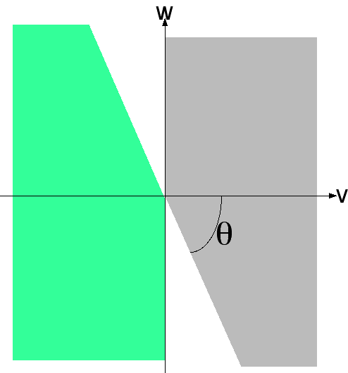
THEOREM 12: The best voting system for 3-candidate elections based on ratings-type ballots (for 100% honest voters, "best" meaning minimizing Bayesian Regret in the RNEM, "honest" meaning they rate the favorite +1, the worst -1, and the other linearly interpolated between based on utility) is the same as range voting except that votes (-1, v, 1) are multiplicatively weighted by W(v) and then the candidate with the greatest weighted sum of scores wins. The magic weighting function is
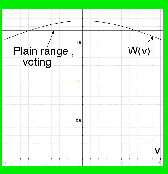
REMARKS: The factor (3π)1/2 is irrelevant since the theorem is equally true with any other positive constant replacing it. This particular value was chosen because it yields unbiased estimates of expected utility (revealed in the proof) but using "1" of course would have been simpler. Some important particular values of this weighting function are
Consequently, the weighting factor W(v) is constant, W(v)≈(π/2)1/231/4≈1.64945 up to a multiplicative error of 21/23-1/4≈1.07457. Therefore this best system is "approximately the same (to within 7.5%) as plain range voting" but not exactly the same.
Proof: A perfect (regret=0) voting system would be "honest utility voting" where each voter rates each candidate with her true utility for his election and the candidate with the greatest summed-score wins. However, range voting, and indeed voting based on scores in any restricted range – for us the range is [-1,+1] – is not perfect because, if the voters cast "normalized" (max=1, min=-1) votes, then these perfect votes necessarily are distorted via scaling and translation. The scaling factor is the "normalization factor"; call its reciprocal the denormalization factor. In the RNEM the expected translation is always 0. Our magic W(v) function in theorem 12 is precisely the expected denormalization factor conditioned on the honest vote being v, |v|≤1, for the middle candidate. To get the formula for W(v) we let u=(1+v)/2 so that 0≤u≤1 and then because of the transformation of variables x,y,z→x,u,y mentioned in the explanations about part 4 of the table of integrals in appendix B, we find
where P(y)=(2π)-1/2exp(-y2/2) is the standard normal density, and where both integrals are over the whole xy plane. Consulting the table of integrals in appendix B we find
Using this W(v), and only it, causes each canddidate's vote total to be the same as his expected utility (conditioned on the votes) hence this voting system is optimal in that it maximizes the expected utility of the winner. QED.
CORRELATIONS: From the explanation of the x,y,z→x,u,y change of variables mentioned in the explanations of the table of integrals in appendix B, we find that the mean square value Sbw of an honest weighted vote in this system is
where
where v=(2z-x-y)/(y-x)=2u-1, and
The integral defining B may be done by doing the two inner (dx and dy) integrals using formulae in section 4 of appendix B, then doing the outer integral (du) by the methods of section 10 of appendix B. The eventual result is
The voteiutilityj correlations (using weighted votes) in the RNEM are
These values all were first computed by high-precision numerical integration but then ways were found to do the integrals in closed form, and finally the formulas and numerical results were verified to coincide to all decimal places. Both Cii and Cij were derived in closed form by using part 4 of Appendix B to do the two inner integrals, then part 10 to handle the outer integration.
The voteivotej correlation (both votes weighted) is
VARIANCES: All three vote-total variances are equal due to candidate-permutation symmetry in our model.
NUMERICAL CONFIRMATION: We computed 20000 triples of standard normal "candidate utility" deviates (7 times). The mean-square (honest weighted) vote in this voting system was found to be 2.18499±0.00055, confirming the theoretical value 2.1849811761.
The mean of the ratio Δ/W, where Δ is the utility difference between the max- and min-utilities in the triple while W is W(v) [where v, -1≤v≤1, is the unweighted vote for the middle candidate] was found to be 0.9976±0.0025, confirming the theoretical claim that weighting by W(v) yields an unbiased estimate of utility (in which case we should have gotten Δ/W=1 in expectation).
We also confirmed the theoretical values of Cii, Cij, and the value "-1/3" numerically to ±0.0005.
THEOREM 13:
Degeneration of rated voting systems in presence of strategic voters
Unfortunately the voting system in the preceding theorem is only "best"
if the voters are honest.
Suppose all the voters instead act strategically as follows:
they give A the maximum and B the minimum possible score, or the reverse
(where A and B are
selected randomly by God before the election as the
two "frontrunners") and then give the remaining candidate C
the exactly intermediate
score (since that maximizes the weight, i.e. "impact,"
of this vote on the crucial A vs B battle).
In that case, our "best rated" system degenerates to become equivalent to strategic
Borda voting (see
remark after theorem 8)
– and that in turn, in the 3-candidate case we are speaking about here,
is equivalent to strategic plurality voting in the sense that both
elect the same winner.
In contrast, plain range voting degenerates with strategic voters to become equivalent to strategic approval voting as discussed in section 5.4, which is considerably better.
Refer back to the regret-computing procedure explained at the start of section 5. We have now computed all the correlations in closed form, and hence are ready to move on to the task of computing Bayesian Regrets. We begin by restating/summarizing our earlier results in the format of the C and D matrices used by that procedure.
Best rated voting system (3 candidates, honest voters): To 8 decimals we find (of course, we actually know exact formulas for all entries for all C matrices in this section; but since many formulas are long we often content ourselves with decimals. See the dictionary table 1 for some of the shorter formulas, and in all cases where the formula isn't in the dictionary, using the known part of C and the known CCT should suffice to determine the missing formulas.)
    [ 0.70844276 -0.35422138 -0.35422138  0.49715518  0.00000000  0.00000000 ]
C ≈ [-0.35422138  0.70844276 -0.35422138  0.08666314  0.48954344  0.00000000 ]
    [-0.35422138 -0.35422138  0.70844276  0.08666314  0.07266879  0.48411985 ]
where the lefthand 3×3 block of this matrix gives the Cij=Correl(votei,utilityj)
from section 6
and the righthand 3×3 block (which is lower triangular) was chosen using
Cholesky factorization
as described in step 3 of the procedure
given at the start of section 5 in order to cause
(CTC)ij
to give the correct vote-vote correlations, i.e.
      [  1   -1/3  -1/3]
CCT = [-1/3    1   -1/3]
      [-1/3  -1/3    1 ].
We also have
    [ 1   0   0 ]
D = [ 0   1   0 ]
    [ 0   0   1 ]
Indeed, from here on the diagonal D matrix (giving the variances)
may always be taken to be (perhaps up an overall scaling factor, which does not matter)
the 3×3 identity matrix, unless otherwise stated.
Range voting (3 candidates, honest voters): From section 5.2 we similarly find
    [ 0.70682747 -0.35341373 -0.35341373  0.50059205  0.00000000  0.00000000]
C ≈ [-0.35341373  0.70682747 -0.35341373 -0.11740835  0.48662889  0.00000000]
    [-0.35341373 -0.35341373  0.70682747 -0.11740835 -0.14910419  0.46322308]
      [1   Q   Q]
CCT = [Q   1   Q] ,    Q = -1/(3Shnrv) ≈ -0.43347748603822207333
      [Q   Q   1]
Best rank-order-based voting system (3 candidates, honest voters) = Borda: From section 5.1 we similarly find – and this is a rank-deficient case so we need to append only two, not three, extra columns to the lefthand 3×3 block of C (but we still can regard the result as 3×6 if we append an extra zero column):
    [ 0.69098830 -0.34549415 -0.34549415  0.53273141  0.00000000 ]
C ≈ [-0.34549415  0.69098830 -0.34549415 -0.26636571  0.46135894 ]
    [-0.34549415 -0.34549415  0.69098830 -0.26636571 -0.46135894 ]
      [  1   -1/2  -1/2]
CCT = [-1/2    1   -1/2]
      [-1/2  -1/2    1 ]
Plurality voting with 3 candidates and honest voters: From section 5.1 we similarly find (another rank-deficient case)
    [  0.59841342 -0.29920671 -0.29920671  0.68033232  0.00000000  ]
C ≈ [ -0.29920671  0.59841342 -0.29920671 -0.34016616  0.58918507  ]
    [ -0.29920671 -0.29920671  0.59841342 -0.34016616 -0.58918507  ]
(Plurality has the same CCT as for Borda immediately above).
AntiPlurality voting with 3 candidates and honest voters: As we remarked in section 5.1 the same C and D matrices arise for antiplurality and for plain plurality voting in N-candidate honest-voter elections with the same N.
Approval with 3 candidates and Honest voters: From section 5.3 we similarly find
    [  0.65147002 -0.32573501 -0.32573501  0.60281027  0.00000000  0.00000000 ]
C ≈ [ -0.32573501  0.65147002 -0.32573501 -0.02492235  0.60229486  0.00000000 ]
    [ -0.32573501 -0.32573501  0.65147002 -0.02492235 -0.02597494  0.60173450 ]
      [  1   -1/3  -1/3]
CCT = [-1/3    1   -1/3]
      [-1/3  -1/3    1 ]
Strategic plurality voting (3 candidates) regarded as strategic Borda: From section 5.5 we similarly find (this is a triply rank-deficient case)
    [ 0.56418958 -0.56418958  0.00000000  0.60281027]
C ≈ [-0.56418958  0.56418958  0.00000000 -0.60281027]
    [ 0.00000000  0.00000000  0.00000000  0.00000000]
and D=diag(1, 1, 0) and
      [ 1   -1   0]
CCT = [-1    1   0]
      [ 0    0   1].
Magic best among the 2 "frontrunners" only (N candidates; 2 chosen at random by God to be labeled "frontrunners"):
    [1 0 0 ... 0]
C = [0 1 0 ... 0]
    [0 0 0 ... 0]
and D=diag(1, 1, 0).
[Note, in both this and the preceding case,
the pseudocode
for computing regrets and wrong-winner probabilities can be modified
slightly to make sure it refuses to elect a non-frontrunner.]
Approval (or Range) with 3 candidates and Strategic voters: From section 5.4 we similarly find (rank-deficient case)
    [ 0.56418958 -0.56418958  0.00000000  0.60281027  0.00000000 ]
C ≈ [-0.56418958  0.56418958  0.00000000 -0.60281027  0.00000000 ]
    [-0.32573501 -0.32573501  0.65147002  0.00000000  0.60281027 ]
      [ 1  -1  0]
CCT = [-1   1  0]
      [ 0   0  1]
"Random winner" with 3 candidates (which by an observation in section 4.1 is equivalent to antiPlurality with strategic voters):
    [0 0 0 1 0 0]
C = [0 0 0 0 1 0]
    [0 0 0 0 0 1]
"Magic Best" and "Magic Worst" with 3 candidates (Magic Best also is called "honest utility voting"):
    [1 0 0]                     [-1   0   0]
C = [0 1 0]       and      C =  [ 0  -1   0]
    [0 0 1]                     [ 0   0  -1]
Here is a dictionary enabling the reader to find exact formulas for many of the numbers stated above as decimals.
| 0.024922 | (π/3-1)([π-2]π)-1/2 |
| 0.266366 | (4-9/π)1/2/4 |
| 0.299207 | (3/8)(2/π)1/2 |
| 0.304142 | (π/3-1)(2π-3)1/2(4π-9)3/2π-1/2(π-2)-1/2 |
| 0.325735 | (3π)-1/2 |
| 0.340166 | (16-27/π)1/2/8 |
| 0.345494 | (8π/3)-1/2 |
| 0.353414 | 31/22ln(3)π-1/4[32π1/2+12-3ln(3)]-1/2 |
| 0.354221 | π[30π-31/29]-1/2 |
| 0.461359 | (12-27/π)1/2/4 |
| 0.497155 | (10π-31/23-2π2)(10π-31/2)-1/2 |
| 0.500592 | [32π+12π1/2-3π1/2ln(3)-72ln(3)2]1/2[32π1/2+12-3ln(3)]-1/2π-1/4 |
| 0.532731 | (4-9/π)1/2/2 |
| 0.564190 | π-1/2 |
| 0.589185 | (48-81/π)1/2/8 |
| 0.598413 | (3/4)(2/π)1/2 |
| 0.602294 | 3-1(2π-3)1/2(4π-9)1/2π-1/2(π-2)-1/2 |
| 0.602810 | (1-2/π)1/2 |
| 0.651470 | 2(3π)-1/2 |
| 0.680332 | (16-27/π)1/2/4 |
| 0.690988 | (2π/3)-1/2 |
| 0.706827 | 31/24ln(3)π-1/4[32π1/2+12-3ln(3)]-1/2 |
| 0.708443 | 2π[30π-31/29]-1/2 |
Using these D- and C-matrices, we can now compute the "wrong"-winner percentages and Bayesian regrets (scaled by V-1/2) for each voting method. The simplest procedure for doing that is P-point Monte Carlo integration:
WrongWinCount←0;  Regret←0;
for(t=1 to P){
   u ← vector of 6 independent standard normal random deviates;
   v ← Cu    (3x6 matrix times 6-vector product, yielding a 3-vector)
   v ← D1/2v    (scales the ith entry of the 3-vector by √Dii)
   i ← 1;   if(v2>v1){ i←2; }   if(v3>vi){ i←3; }
   j ← 1;   if(u2>u1){ j←2; }   if(u3>uj){ j←3; }
   (Now i maximizes vi while j maximizes uj)
   if(i≠j){
     WrongWinCount ← WrongWinCount + 1;
     Regret ← Regret + uj - ui;
   }
}
print("Wrong Win Percentage ≈ ", 100.0*WrongWinCount/P);
print("V-1/2Bayesian Regret ≈ ", Regret/P);
which prints values arbitrarily near to the correct ones
with probability→1 in the P→∞ limit.
We can however also compute the Wrong Win Percentage and Bayesian Regret
analytically in terms of Schläfli functions S6
and pure-linear moments, respectively. Both are described in
Appendix C where it is shown that closed
formulas for the latter always exist; the former also have closed forms in every
rank-deficient case; in both cases dilogarithms may be needed. (If trilogarithms are
permitted, then every entry has a closed form.)
The following table summarizes the results. It gives the Wrong Win Percentage and Bayesian Regret for all the voting methods shown, in 3-candidate RNEM elections in the V→∞ limit.
Notes on the table: We list voting systems in best-to-worst, i.e. increasing-regret, order. All (≤7)-digit numeric values were computed using P≥1.6×10¹²-point Monte Carlo integration using the pseusocode above with standard-error estimates taken as the sample standard deviation of 5 subsample-means (each subsample with P/5 points) divided by √5. This accuracy is estimated to be ±k units in the last decimal place, where k is given in parentheses after the number. We sped up the program by about a factor of 10 by using the following trick. The main timesink in the code is the generation of the 6-vector of normal random deviates, which we do using the Box-Muller polar method. (See discussion of normal deviate generation in appendix D. Substantially faster methods for generating normals are available, namely the Marsaglia-Tsang "ziggurat" method and the Wallace-Brent all-real methods, but I avoided the former due to worries that I might introduce "bugs" and the latter due to worries about its statistical quality.) We therefore generate one such 6-vector but then use it 16 times via considering all ways to make an even number of sign changes in the first 5 coordinates. This 16× trick not only speeds up the computation; it also appears to increase its accuracy by decreasing variance while leaving expectation value unaltered (i.e. these points are "better than random").
About the Monte Carlo code: As a smaller-scale check on the Monte Carlo code, we ran it with 100 times fewer points using Marsaglia's MWC1038 generator of period>233245. (That should yield exactly 1 fewer digits of accuracy.) We also did this again, the second time with Marsaglia's KISS generator of period>2124; and finally a third time using the generator (due to Brent and Marsaglia, call it "BM256")
which directly returns uniform real numbers in [0,1) without requiring any conversion from integers. All three sanity checks worked in the sense that their statistical errors were within expected bounds – but unfortunately, their results disagreed! Specifically, KISS and MWC1038 agreed, but exhibited small but reproducible systematic disagreements with BM256. I suspect most or all of the reason was the fact that KISS and MWC1038 generate 32-bit random words while BM256 generates random 52-bit reals (the number of bits in an IEEE standard real mantissa). The simple solution to this unacceptable problem was to combine the outputs of the MWC1038 and BM256 generators by mod-1 addition to get a result at least as random as either, and that was the underlying generator used for the final, large, run.
The tabulated values with 9 or more digits were computed using closed formulas. In principle all values could have been computed with closed forms, but the formulas can get large, see appendix C's of discussion of formula length.
| Voting method | "Wrong winner" percentage | V-1/2Regret |
|---|---|---|
| Magic Best | 0 | 0 |
| BRBH=Best ratings-based (Honest voters, see sec. 6) | 18.70338(6)% | 0.0674537(2) |
| Honest Range | 22.35938(6)% | 0.0968636(3) |
| Honest Approval (mean as threshold) | 25.86333(3)% | 0.1300873(4) |
| Best rank-order-based (Honest Voters)=Borda | 25.86335(4)% | 0.1300876(2) |
| Strategic Approval (=Range, see theorem 13) | 30.98197(3)% | 0.1863856(2) |
| Honest Plurality=AntiPlurality | 33.99984(3)% | 0.2260388(4) |
| Magic best among the 2 frontrunners only | 1/3≈33.3333333% | |
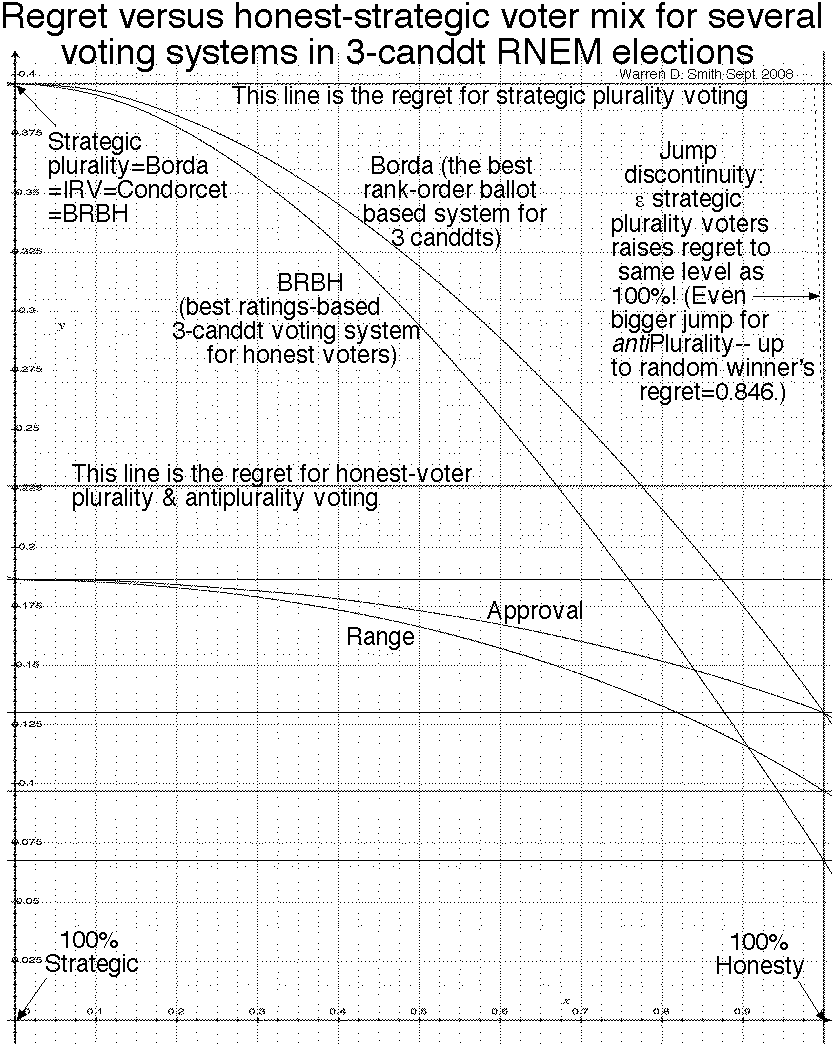
| Strategic Plurality (=Borda=IRV=Condorcet=BRBH, see theorems 8 & 13) | 45.43326(5)% | (3/2)π-1/2-21/2/π≈0.3961262173 |
| Random winner=Strategic AntiPlurality | 2/3≈66.6666667% | (3/2)π-1/2≈0.8462843754 |
| Worst winner | 100% | 3π-1/2≈1.6925687506 |
NUMERICAL CONFIRMATION:
I compared the tabulated numbers (as well as
our theoretical regret 0.1140314256V1/2
from
REMARKABLE COINCIDENCE: The regrets (and the wrong-winner probabilities too!) for honest approval and Borda voting agree to within about a part in 100,000. This astonished me and led me to ask whether, in fact, they are equal.
Approval clearly seems better than Borda in the sense that approval voters get to indicate one of two possible scores for their middle-choice candidate, whereas Borda voters cannot transmit any information about him. (In both systems, honest voters behave exactly the same about their top and bottom choice candidates, so the only difference is the middle choice.) But approval forces voters to exaggerate their views of the middle candidate to be "equal" to the best or worst – a distortion which clearly makes approval suboptimal for honest voters. The amazing thing is that evidently these positive and negative effects exactly cancel!
As we shall see in the next theorem, they are equal.
This was initially mysterious. A sufficiently determined reader could, using our closed formulas, compute both BRs to 500 significant figures, then verify their equality. (Also, even without the closed formulas, one could still get considerably greater accuracy by using better methods for numerical integration than Monte Carlo, see Stroud 1971.) However, even 500-place agreement still would not prove exact equality. One could try to simplify both formulas to a common canonical form... but unfortunately at present no algorithm is known to simplify formulas involving polylogarithms (even dilogs) to canonical forms – and I can say from personal experience that MAPLE is exceedingly incompetent at it – and since these formulas are very long (see appendix C's of discussion of formula length), this proof would also be enormous even if it could be done.
So those brute-force proof-ideas seem unpromising. But a more elegant attack works.
THEOREM 14 (Borda and Approval "geometrically the same"): Borda and Approval voting have the exact same regrets and wrong-winner probabilities (for honest voters in the 3-candidate random normal elections model).
Proof: The proof idea in 5 words is: "Don Saari's planar geometrical picture." (See figure. This idea is in his book Basic geometry of voting.)
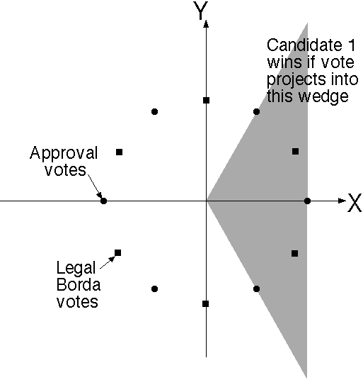
Although it seemed like 3-candidate Borda and Approval votes v are 3-dimensional, really they only are 2-dimensional because it is OK to view everything projected into the plane v1+v2+v3=0.
In this plane, the 6=3! allowed Borda votes
are the vertices of a regular hexagon. (Different weighted positional systems would lead to irregular hexagons.)
The 6=23-2 non-silly approval votes (rescaled and translated to lie on the v1+v2+v3=0 plane)
also form the vertices of a regular hexagon.
Up to a scaling by a factor of √3 (which cannot matter) and a rotation by 30 degrees, they are the same hexagon.
If we project the lefthand 3×3 blocks of the Borda and Approval honest-voter C matrices from section 7 (where Cij is the voteiutilityj correlation) into a 2-dimensional XY plane, then (up to scaling) these 2×3 matrices result:
[6      -3       -3     [6(4π-9)]1/2            0]
[0      3√3    -3√3     0            [6(4π-9)]1/2]
where the reader may check that the same matrix arises for either Borda or Approval voting. (Only pay attention to the leftmost 3 columns of the matrix for the moment.) Now due to the hexagonal symmetry, the vote-distribution in this XY plane must be a circularly-symmetric normal distribution, not elliptical. This vote distribution arises (up to a scaling factor) by generating a vector u of standard normal deviates, then computing the matrix-vector product Cu. If u is 3-dimensional, then the reader may check that a 2-dimensional perfectly circularly-symmetric normal distribution indeed results from this C. In order to make the vote distribution come out right, we also need to add more noise, which effect is got (just as in the correlation-based procedure before, in the step where we added "extra columns") by adding extra components to the u vector and extra columns to the C-matrix. These extra columns, in order not to destroy the perfect circular symmetry (and assuming they form a triangular matrix, as we know from earlier work they must), must wlog form a multiple of the 2×2 identity matrix. (In fact, by, e.g, projecting the full Borda 3×5 matrix we can show it is exactly the multiple shown in the rightmost two columns, but we will not need this fact for the purposes of the present proof.)
Honest Borda voters decide which one of the 6 legal votes to cast, by seeing which of 6 wedge-shaped regions (each with apex angle 60° forming an infinite "pie") the 2D-projected (u1, u2, u3) lies in. Honest approval voters instead examine the 12-wedge pie got by bisecting every Borda pie-wedge, and there is a fixed 2-to-1 map from pie wedges to votes. The Borda voters of course may also be viewed as consulting the 12-wedge pie and using a (different) fixed 2-to-1 map.
The only difference between approval and Borda is the 30° angle by which the hexagon of legal votes is rotated relative to this (fixed) pie. However, since the wedge-angles of the 12-wedge pie are each 30°, this really is no change at all. If we agree to rescale the Borda and Approval votes to make their circularly-symmetric-normal vote-distributions in the XY plane identical, the pictures actually are the same.
It therefore follows (since their scalings must be the same) that both the lefthand and the righthand blocks of the 2×5 C-matrices are the same for both Borda and Approval.
Therefore, the integrals defining RNEM Bayesian Regret and wrong-winner probability, also are the same. [Specifically, the integrals are over the region of 5-space (u1, u2, u3, u4, u5) where (say) candidate 1 wins because X>|Y|tan(30°) where (X, Y)T=Cu, but u2>u1 and u2>u3 so that candidate 2 was the greatest-utility winner. The integrand is the normal density times u2-u1 for Regret (or just times 1 for wrong-winner probability). Finally we need to multiply by a factor of 3!=6 to count all symmetric images of this scenario.]
The proof is complete. QED.
NUMERICAL CONFIRMATION: When we explicitly write the 5-dimensional integral representations of the wrong winner probability≈25.863% and Bayesian Regret≈0.13009 deduced in the above proof, we get (after the additional trivial change of variables u1=x2-x1, u2=x2, u3=x2-x3, u4=x4, u5=x5, and using the fact that cot30°=√3)
where F'(y)=(2π)-1/2exp(-y2/2) is the standard normal density and the integral is over the region
and
The right hand side instead gives ≈0.13009 if its integrand is multiplied by x1. These two numerical values were obtained by numerical integration (via ACM TOMS algorithm 698) of the outer 4 integrals (with ±∞ truncated to ±6) after a symbolic integration (using erf) of the innermost integral. Their agreement with the values found earlier using Monte Carlo integration of the original form of the integral, constitutes numerical confirmation both of the symbolic manipulations inside the proof, and of my Monte Carlo program.
It is possible to reduce the whole 5D-integral to close form using the Schläfli function theory in appendix C. As an experiment, I asked MAPLE to do this for the wrong-winner probability, but the resulting closed form was many pages long and when MAPLE was asked to simplify it it went into an (apparently) infinitely-long think.
REMARK: The amazing equalities in theorem 14 only hold for ≤3 candidates. (Borda would have lower regret than approval in ≥4-candidate RNEM elections with honest voters, albeit approval does better with strategic voters.)
References for Section 7:
Richard P. Brent: Some Comments on C.S. Wallace's Random Number Generators, The Computer Journal 51,5 (2008) 579-584.
Pierre L'Ecuyer & Richard Simard: TestU01: A software library in ANSI C for the empirical testing of random number generators, ACM Transactions on Mathematical Software 33,4 (August 2007) Article 22.
George Marsaglia: Random Number Generators, J. Modern Applied Statistical Methods 2,1 (May 2003) 2-13.
Donald G. Saari: Geometry of Voting, Springer 1995.
G.Marsaglia & Wai Wan Tsang: The ziggurat method for generating random variables, J. Statist. Softw. 5,8 (2000) 1-7. [There are two slight bugs in their code for random normals. Low-order bits from the same random integer used to provide the sample, are re-used to select the rectangle – causing a slight correlation which causes the generator to fail high-precision tests. Getting those bits from an independent random word fixes that. Also, a further even smaller flaw is that using 32-bit random integers is not really sufficient for generating 52+-bit random-real normals, so their output is artificially "grainy."]
Arthur H. Stroud: Approximate Calculation of Multiple Integrals, Prentice Hall, 1971.
D.B.Thomas, W.Luk, P.H.W.Leong, J.D.Villasenor: Gaussian Random Number Generators, ACM Computing Surveys 39,4 (Oct. 2007) Article 11. [Concludes Ziggurat and Wallace are the best; 2-to-7 times faster than Polar method.]
What if some fraction F of the voters are honest while 1-F are strategic? More generally, we can consider a K-component voter mixture where fraction Fk≥0 for k=1,2,…,K have behavior k, with ∑1≤k≤KFk=1.
THEOREM 15 (Multicomponent voter mixtures): The same Monte-Carlo procedure works as before to compute Bayesian Regret from the D and C matrices for the voting systemss except that instead of the lines that compute
we instead compute
where (for k=1,2,…,K)
We warn the reader that this only necessarily works for nonsingular voting systems where all the entries of the C and D matrices are well defined. (Strategic Plurality and antiPlurality voting are singular as was explained in section 5.5; and we shall explain what happens for them in theorem 17.)
Again, instead of Monte Carlo we can simply compute the corresponding integrals as before. Again we get Schläfli and moment functions (see appendix C) just as before. Although the method in theorem 15 has the virtue of simplicity (the proof should be obvious – the given formula makes the correlations, variances, and expectation value come out right; and because of the properties of multidimensional normal distributions, that's enough – and the Monte-Carlo procedure is very simple) it is poor for analysis purposes because it unfortunately multiplies the dimensionality of the integrals by K. That difficulty is illusory; really the dimensionality is not increased at all.
THEOREM 16 (Dimension non-increase for voter mixtures):
The K-times-higher dimensional integrals arising for voter
Proof sketch: The votei-utilityj correlations (i.e. the correlations between yi and uj in the Monte Carlo pseudocode) are easily worked out exactly from the component matrices. These will be used to fill in the lefthand N×N block of the C matrix. Then the righthand block will be computed via Cholesky as before to make the votei-votej correlations come out right (those too are easily worked out exactly), and as before this requires at most N extra columns to be adjoined to the C matrix. Finally, the vote variances (in y) too are easily worked out exactly and used for the entries of the D matrix. QED.
Due to this non-increase, we still have closed forms using low-dimensional Schläfli and moment functions (see appendix C) for any voter mixture.
THEOREM 17 (Discontinuities): For plurality voting in the RNEM, introducing a fraction ε of strategic voters into the mix, for any ε>0 no matter how small, causes the regret to jump discontinuously to the same value as plurality with 100% strategic voters. The same thing happens with antiplurality voting.
Proof: With ε fraction strategic voters who (for plurality voting) always vote for one of the two "frontrunners" (whichever they perceive to be the "lesser evil") and zero for every other candidate, the net result will be a boost in vote total by an amount≥Vε/2, for the most popular frontrunner. This, in the V→∞ limit, far exceeds the differences of order (1-ε)V1/2 among all the other candidates arising from the honest votes. It therefore, with probability→1 in the V→∞ limit, forces the top frontrunner to win, i.e. the same result as with 100% strategists (at least, assuming the strategic and honest voters have the same utilities independently, and the RNEM does assume that; and we are implicitly using well known tail properties of the normal distribution and central limit theorem). Similarly for antiPlurality voting, the non-frontrunner with the fewest honest antivotes always wins for any ε>0 with probability→1 in the V→∞ limit. QED.
REMARKS:
Using theorems 14-16, I computed the regret curves for our voting methods. Compatible scalings for the D matrices arise from the following:
OBSERVATIONS:
Philosophical note: Also, even if somebody truly did the job, one would have to wonder, in view of the complexity of their software, whether that proof would really generate more confidence than our non-proof. I.e. consider a hypothetical graduate student who announced "I wrote a 5000-line computer program to do all the formulas, symbolic differentiation, and interval arithmetic, and it has now genuinely completed the proof! My program sits on top of a 1,000,000-line commercial symbolic manipulation system with secret code, a 2,000,000-line operating system, a 300,000-line compiler, and a secret computer design involving 1,000,000,000 transistors, all of which depend upon the validity of quantum physics and correctness of manufacturing, and all of which, in fact, are known to contain bugs... So trust me." At some point, debates over the "logical validity" of such proofs begin to resemble arguments about how many angels can dance on the head of a pin.I also made a plot of the derivatives of these curves, which is not shown because it is about 50 times less accurate. Nevertheless, its accuracy is sufficient for confidence in (i), although it still leaves room to doubt (ii) and (iii). The plot also indicates all the smooth curves have |derivatives|≤0.6 everywhere, which would imply that at most 12 plot points suffice for a rigorous proof of our Main Result that range is everywhere-superior to Borda. (A line segment joining the regrets for "worst winner" and "best winner" would, in contrast, have slope≈1.69.)
Lazy man's interval arithmetic: The mechanical task, outlined above, of using closed formulas and interval arithmetic to prove the Main Result, is painful and philosophically debatable and so I did not do it. The question then arose: was there some less-painful way to get the same effect (or nearly so)? Here are some answers:
It might be possible to justify (c) with the aid of the following conjecture. Each of our two plotted curves (Borda and Range) are defined by two C-matrices, each of which has bounded |entries|, and determinant(CCT) bounded away from 0. We may now consider replacing these two matrices by the worst possible such matrix pair, i.e. leading to a curve with the maximum possible |derivative|. Here we can instead of taking derivatives with respect to the honesty-fraction F, 0≤F≤1, employ other variables such as θ where 2F=1+cosθ and 0≤θ≤π. I conjecture that with some appropriate choice of variable the worst possible matrix-pair arises from "magic best winner" and "magic worst winner." If so, one could easily see that using 1000 plot points (which I did) would be more than sufficient to get a rigorous proof.
In view of this, even though we admittedly have not undertaken the maximally-magnificent interval-arithmetic calculation, we claim the cruder calculation we did do nevertheless would suffice for full rigor provided we trust the random number generator, we accept a "probabilistic proof" with a tiny and rigorously boundable failure probability, and we accept or prove the above conjecture.
Probabilistic proofs are well-accepted nowadays, e.g. the Atkin-Larson probabilistic primality test, which either proves an input number P is composite, or proves that either P is prime or the used random bits were exceedingly unlucky (i.e. again we have an exponentially tiny rigorously boundable failure probability).
In summary: Despite these inadequacies, for the purposes of political scientists rather than ultrapure mathematicians, the issue is already settled: claims #1 and #2 i, ii, iii are true accurate to a part in a thousand. So be happy.
Finally, we observe that the BRBH system, although it is better than range voting, only is better if the percentage of honest voters exceeds about 91%. Otherwise it is worse, and usually a lot worse. 91% is large enough that I think there should be no doubt that, for practical purposes, range voting is superior even to BRBH. Range and especially approval voting are both good for honest voters and comparatively insensitive to voter strategizing.
When considering computing "regrets" and "wrong-winner probabilities" from our 3×6 C-matrices, there are 6 hyperplanes that matter in the 6-dimensional space of vectors u. Their equations are:
These hyperplanes define a polytopal cone in the 2N-dimensional space of vectors u (since the vote-vector v can be regarded as a linear function of u inside the Monte-Carlo integration procedure from section 7). In fact, however, this cone is divisible into (N-1)N interior-disjoint simplicial cones, each defined by only 2(N-1) hyperplanes. Namely, in our case N=3, a typical simplex is
As an immediate consequence, therefore, we see that all the "wrong-winner probabilities" arising from 3×6 C-matrices can be expressed using dilogs without need of trilogs.
Furthermore, the integration to find the regrets is over the same disjoint union of simplicial cones, but instead of the integrand being a constant it is now a pure-linear function within each simplex (namely proportional to u2-u1 in the "typical tetrahedron" above). This integral may be done (using the methods in appendix C) using only arctrig without needing dilogs!More generally, for N candidates, using C-matrices that are N×2N, we have
THEOREM 18 (dimensionality below what one might think): In N-candidate RNEM elections where our correlation-based procedure is applicable to find regrets, those regrets are expressible as a sum of (N-1)N noneuclidean simplex (2N-4)-curved-dimensional volumes (i.e. Schläfli functions S2N-3), each corresponding to a region where "j wins but k was the max-utility candidate"; and the wrong-winner probabilities are expressible as a sum of (N-1)N noneuclidean simplex (2N-3)-curved-dimensional volumes, i.e. Schläfli functions S2N-2 in the notation of appendix C.
The dihedral angles between the just-discussed hyperplanes (ignoring 90° dihedrals, and where the reader is warned that angles θ would have to be replaced by the supplementary angles π-θ if the other side of one hyperplane is regarded as the "inside") are:
       [Ca-Cb]·[Cj-Ck]
arccos(--------------)
       |Ca-Cb|·|Cj-Ck|
(between the
va=vb and
vj=vk hyperplanes, where Cr
denotes the rth row of C)
       [Ca-Cb]j - [Ca-Cb]k
arccos(------------------)
           |Ca-Cb|  √2
(between the
va=vb and
uj=uk hyperplanes).
References for Section 8:
G.Alefeld & J.Herzberger: Introduction to Interval Computations, Academic Press, 1983.
A.O.L. Atkin & R.G. Larson: On a primality test of Solovay and Strassen, SIAM J. Comput. 11,4 (1982) 789-791.
Andreas Griewank: Evaluating Derivatives: Principles and Techniques of Algorithmic Differentiation. SIAM (Frontiers in Applied Mathematics #19) 2000.
R. Hammer, M. Hocks, U. Kulisch, D. Ratz: Numerical Toolbox for Verified Computing I: With Algorithms and Pascal-XSC Programs, Springer-Verlag, Berlin, 1994.
T.Hagerup & C.Rüb: A guided tour of Chernoff bounds, Information Processing Letters 33,6 (1990) 305-308.
Eldon Hansen & G. William Walster: Global Optimization using Interval Analysis (2nd ed.) Marcel Dekker, New York, 2004.
Ramon E. Moore: Interval Analysis, Prentice Hall, Englewood Cliffs, N.J., 1966.
Ramon E. Moore: Methods and Applications of Interval Analysis, SIAM, Philadelphia PA 1979.
Miodrag S. & Ljiljana D. Petkovic: Complex Interval Arithmetic and Its Applications. Berlin: Wiley, 1998.
Louis B. Rall: Automatic Differentiation: Techniques and Applications, Springer (Lecture Notes in Computer Science #120) 1981.
The mathematician awoke and saw there was a fire. He ran over to his desk, began working through theorems, lemmas, and hypotheses, and after a few minutes, put down his pencil and exclaimed triumphantly "I have reduced the matter to previously solved problems, thus proving that I can extinguish the fire!" He then went back to sleep.
This paper's accomplishment somewhat resembles the above joke. For 3-candidate voting systems in the RNEM, we have by plotting two curves demonstrated that range voting is superior (measured by Bayesian Regret) to the best rank-order voting system, for either honest or strategic voters, or any mixture (and approval voting also is thus-superior, except at 100% honesty where it equals but does not better Borda). But, strictly speaking, this was not a proof, because it does not exclude the possibility that through some miracle-conspiracy of arithmetic roundoff errors, or some miraculous incredibly sharp and high spike in one of the plotted curves, that the lower-regret curve might somehow manage to avoid being lower everywhere.
However, like the mathematician in the joke, we have proven that fire can be extinguished. Specifically:
It would probably be possible for a graduate student to now do the final step in about 1-10 weeks of computer programming and debugging. However, one has to ask whether it would really be worth that effort, see "philosophical note" in section 8.
I have been asked why I claim that Bayesian Regret is the only correct way to objectively measure voting system quality. I'm tempted just to respond that statisticians over 200 years have pretty much come to a consensus that Bayesianism is the unique philosophically correct approach to statistics and objectively comparing the quality of different statistical estimators generally, and so ask them, not me. (See Jaynes 2003, Sivia-Skilling 2006, Robert 2001, Berger 1993.) I also could respond that Bordley and Merrill both independently invented the Bayesian-Regret framework for comparative evaluation of voting systems (and before me), so again, ask them, not me. This argument was fought, and won, long ago, with a strong majority consensus being reached in every scientific area except economics, where (for obscure historical reasons) holdouts against the whole notion of "utilities" still are frequently encountered even in the 21st century.
For a somewhat deeper response, aimed particularly at those people, see /OmoUtil.html
Our Bayesian Regret framework and overarching technique for determining "best voting systems" in no way depend on the RNEM. Anybody who prefers a different and more-realistic model of voters is free to use it instead. (Our 1999-2000 computer results indeed did employ many other models and the superiority of range voting over all the rank-order-ballot based competitors tried, was very robust across models; and the follow-up paper "part III" will be able to make some rigorous statements about regrets in certain other interesting models.)
I did not use the RNEM because of a delusion it was a highly-realistic model of elections. The two most important ways it is unrealistic are:
is more realistic in the latter respect. The reasons this paper focused on the RNEM are that it is
The so-called "impartial culture" (IC) is the degenerate case of the RNEM arising from specializing to rank-order-ballot voting systems. (IC is: all candidate-orderings equally likely by each voter independently.) It has been heavily studied by many political-science authors. Despite IC's unreality, my personal experience is that the probabilities predicted by the IC model for various kinds of voting pathologies, usually agree tolerably respectably with attempts to measure frequencies of those pathologies in real life (where note that such real-life measurements usually are difficult, debatable, and noisy); see table 3.
| Phenomenon | IC Probability | DM Prob'y | Approximate frequency in real life |
|---|---|---|---|
| 3-canddt IRV is nonmonotonic | (14.7=12.2+2.47)% (two disjoint kinds of nonmonotonicity) | (3.22=2.17+1.05)% | About 20% based on the 9 Louisiana governor elections 1995-2007 |
| In 4-canddt Condorcet elections, adding new bloc of co-voting voters makes election result worse for them | Roughly (0.5 to 5)% depending on Condorcet flavor | ? | ? |
| 3-canddt IRV eliminates a Condorcet Winner | 3.71% | 3.23% | Apparently 9 CWs eliminated in the 150 federal IRV elections in Australia 2007. (But in "1-dimensional politics" models this phenomenon is more like 25-33% common.) |
| 3-canddt plurality voting winner same as "plurality loser" | 16.4% | 9.25% | Seems in right ballpark |
| 3-canddt IRV voting winner same as "IRV loser" | ≈2.5% | 1.7% | ? |
| 3-canddt IRV elections where adding new co-voting bloc causes election winner to worsen in their view | 16.2% | 7.4% | Apparently about 40% based on the 9 Louisiana governor elections |
| 3-canddt IRV voting "favorite betrayal" situation where a bloc of co-voting C voters can improve election winner in their view by not voting their favorite C top (does not count nonmonotone situations where this makes C win) | 20.2% | Apparently about 40% based on the 9 Louisiana governor elections | |
| 3-canddt election features Condorcet cycle | [3arcsec(3)-π]/(2π)≈8.78% (Guilbaud 1952 in footnote; see also Gehrlein 2006) | 1/16=6.25% | About 1% (Tideman 2006's theoretical extrapolation from real-life data); some models of "1-dimensional politics" predict 0% |
| "Majority-top winner" exists in 3-canddt election | 0 | 9/16=56.25% | Happened for 50% of Australian federal IRV seats in 2007 election and 44% of the 9 Louisiana governor elections. |
The IC estimates in the top part of the table seem to be working reasonably well, in particular as well or better than the Dirichlet model, but the bottom two lines disagree noticeably with reality. Regenwetter et al explain, in chapter 1 of their book, theoretical reasons why IC would be expected to maximally overestimate the probability of "Condorcet cycles" in 3-candidate elections. And indeed the IC theoretical prediction 8.78% is a large overestimate of the real-life rate of approximately 1% (albeit Condorcet cycles seem fairly common in legislative votes since they are intentionally created as part of "poison pill" legislative tactics). Even worse, "majority-top winners" occur zero percent of the time in IC 3-candidate elections in the V→∞ limit but actually are quite common in real life. The "Dirichlet model" predicts 56.25%.
The reader may ask "why have you only focused on 3-candidate elections? What about 4, 5, and 6?" The answer is that the techniques in this paper will easily permit the reader to calculate the honest-voter regrets to, say, 4-digit accuracy and thus produce a convincing non-proof that range voting is superior to the best rank-order system, with honest voters, for those numbers N of candidates also. This is done in the follow-up paper Part II.
I focused on the 3-candidate case here because it is specially nice because closed formulas exist and hence this non-proof can be converted into a genuine proof. (Also, of course, 3 is the simplest and most important nontrivial number.) We know from section 8.2 that closed formulas involving dilogs will also be attainable for 4-candidate regrets.
An obvious question is to determine more closed formulas. The reader should, with enough work, be able to use our techniques to write down closed formulas for all the regrets and wrong-winner probabilities in the big results table, as well as extending that table to cover 4-candidate elections. The key word is "enough" work, and a question is whether those formulas can be simplified sufficiently that they become attractive. These questions are more of aesthetic than genuine interest – just knowing the answer accurate to 3 digits seems good enough for any political science purpose, so trying for a beautiful exact formula has no objective importance. Because I am a mathematical aesthete, though, I apologize that I have not found as many such formulas as I should. Anybody expert with symbolic manipulation systems ought to be able to find more than I.
Some problems of more general and genuine interest are to develop automated techniques for simplifying formulas involving dilogarithms, and to understand whether and when Schläfli functions in N dimensions can be expressed in terms of nice 1-dimensional functions (see appendix C).
Another question: "what about voting systems where the 'votes' are something other than pure rank-orderings of the candidates, or other than numerical ratings?" As a concrete example of such a voting system (suggested by Ivan Ryan), consider Condorcet voting but the votes are not plain rank-orderings – voters also are allowed to employ one ">>" in the order, for example
Then Ryan's proposal was that any A>B relationship on a ballot which included a ">>" somewhere in the path, should count as 2 votes. (Or your favorite constant in place of "2"; this could be tuned to optimize performance.)
Then the pairwise table is computed as per the usual Condorcet prescription and we attempt to find a Condorcet winner as usual.
This allows a voter to express (to some degree anyway) "strength of preference." Also, because it moves outside of the usual "pure rank order" framework by allowing a more general kind of vote, it evades our mathematical results indicating that range voting is superior regret-wise to every rank-order system.
Our mathematical techniques still would allow analysing voting systems with this kind of "one->>" ballot and finding the best such system and its regret. Perhaps range voting still would be superior to the best such system, but future investigators will have to do that analysis.
Another question is: "what about other statistical/political models besides RNEM (such as D-dimensional politics models, etc)?" Can future authors prove analogous results to ours in those models? With the help of some fortuitous miracles we are able to accomplish that in some cases. That will be explained in the follow-up paper "part III."
References for section 9:
James O. Berger: Statistical Decision Theory and Bayesian Analysis 2nd ed. Springer (Series in Statistics) 1993.
William V. Gehrlein: Condorcet's paradox, Springer 2006.
G.Th.Guilbaud: Les théories de l'intérêt général et le problème logique de l'agrégation, Economie Apliquée 5,4 (1952) 501-584.
E.T. Jaynes: Probability theory: The logic of science, Cambridge Univ. Press 2003.
M.Regenwetter, B.Grofman, A.A.J.Marley, I.M.Tsetlin: Behavioral social choice: probabilistic models, statistical inference, and applications, Cambridge University Press, New York 2006.
Christian P. Robert: The Bayesian choice: From decision-theoretic foundations to computational implementation, Springer (texts in statistics) 2001.
Devinderjit Sivia & John Skilling: Data Analysis: A Bayesian Tutorial, Oxford University Press (2nd edition 2006).
Nicolaus Tideman: Collective Decisions and Voting: The Potential for Public Choice, Ashgate 2006.
I thank Drs. Steven J. Brams, Nicholas Miller, Steve Omohundro, Marcus Pivato, and Alan T. Sherman for stylistic and publication advice and/or literature references, and Rick Carback for donating computer time.
Denote the expected value of the kth greatest of N independent standard normal deviates, by Gk(N). Of particular interest is G1(N), the expected value of the maximum of N independent standard normal deviates:
Proof: The first expression should be immediate from the definition and the fact that the negated minimum is the same as the maximum (in expectation) due to even symmetry. It is actually valid for any even-symmetric differentiable probability density F'(y) well enough behaved when y→±∞, although we are only interested in the standard normal density here. Then the second arises because it is trivially equivalent to
In the limit N→∞, we have
In addition to the expectation value, it also is possible to compute the variance of the maximum of N independent standard normal deviates. It is
[Proof sketch: These arise by combining Hall 1979 with section 9 of our table of integrals in appendix B.]
One could go further and indeed compute the mean, the variance, and any particular moment asymptotically when N→∞ as an asymptotic series expansion in N (these expressions were merely the first-order terms in those series) by using the "saddlepoint method" (Bender & Orszag 1978) of asymptotic analysis of our first integral expression.
| N | G1(N) | N | G1(N) |
|---|---|---|---|
| 1 | 0 | 11 | 1.58643635190800 |
| 2 | π-1/2≈0.56418958354775 | 12 | 1.62922763987191 |
| 3 | (3/2)π-1/2≈0.84628437532163 | 13 | 1.66799017704913 |
| 4 | 3π-1/2[1/2+π-1arcsin(1/3)]≈1.02937537300396 | 14 | 1.70338155409998 |
| 5 | (5/2)π-1/2[1/2+(3/π)arcsin(1/3)]≈1.16296447364052 | 15 | 1.73591344494104 |
| 6 | 1.26720636061147 | 16 | 1.76599139305479 |
| 7 | 1.35217837560690 | 17 | 1.79394198088269 |
| 8 | 1.42360030604528 | 18 | 1.82003187896872 |
| 9 | 1.48501316220924 | 19 | 1.84448151160382 |
| 10 | 1.53875273083517 | 20 | 1.86747505979832 |
| 200 | 2.74604244745115 | 2000 | 3.435337162 |
| 20000 | 4.01878926 | 200000 | 4.53333091 |
A more general formula is
where 1≤k≤N. [This is valid for any probability density F'(y), not just the particular standard normal one we are interested in here, and arises because the kth smallest of N i.i.d. random deviates has F(y) that is Beta(k, N+1-k)-distributed.] Of course by symmetry
One reason for the pre-eminent importance of the G1(N) is that all the other Gk(N) can be computed in terms of them alone, via the recurrence
[Proof sketch: consider the kth greatest among N-1 random points, then add an Nth
point. With probability k/N it becomes the
Consequently, for example,
However, the reader is warned that this recurrence is numerically unstable when used in the forward direction.
Define
This can also be used (instead of G1(N)) as the "master" quantity from which all the Gk(N) can be derived via the above linear recurrence. As a consequence of Jensen's inequality
where ◻N→1 in the N→∞ limit since the sum becomes a Riemann integral.
The theory exposited in appendix C on Schläfli functions and moments shows that closed formulas (but now involving dilogarithms as well as more elementary functions) also exist for all the G(6), and G(7), and if we allow also trilogarithms then closed forms exist for all the G(8) and G(9) too. [I used the symbolic manipulation system MAPLE9 to determine G1(6), ◻6, and ◻7, but will not state these results since each was approximately 4 pages long. Quite possibly much shorter simplified forms exist, but both MAPLE9 and every other contemporary symbolic manipulation systems are almost incapable of simplifying expressions containing dilogs.]
| N | Gk(N) for k=N, N-1, ..., 2, 1 | ◻N=∑1≤k≤N[Gk(N)]2/N |
|---|---|---|
| 1 | 0 | 0 |
| 2 | -0.56418958354775629, 0.56418958354775629 (Plurality) | 0.31830988618379067=1/π |
| 3 | -0.84628437532163443, 0, 0.84628437532163443 (Borda) | 0.47746482927568600=3/(2π) |
| 4 | -1.0293753730039641, -0.29701138227464533, 0.29701138227464533, 1.0293753730039641 | 0.57391470987387290=9[π2-4πarcsin(1/3)+20arcsin(1/3)2]/(4π3) |
| 5 | -1.1629644736405196, -0.49501897045774221, 0, 0.49501897045774221, 1.1629644736405196 | 0.63901205922520556=5[5π2-36πarcsin(1/3)+180arcsin(1/3)2]/(8π3) |
| 6 | sym, 0.20154683380170425, 0.64175503878576119, 1.2672063606114713 | 0.68609420546552530 |
| 7 | sym, 0, 0.35270695915298243, 0.75737427063887269, 1.3521783756069044 | 0.72182981266275276 |
| 8 | sym, 0.15251439950692319, 0.47282249494061799, 0.85222486253829092, 1.4236003060452778 | 0.74993670036986136 |
| 9 | sym, 0, 0.27452591911246175, 0.57197078285469610, 0.93229745673360373, 1.4850131622092370 | 0.77265726588235093 |
| 10 | sym, 0.12266775228433806, 0.37576469699787754, 0.65605910536476120, 1.0013570445758144, 1.5387527308351729 | 0.79142718641334414 |
One may also estimate the variance corresponding to Gk(N) for other k. For example [by using the known connection to the Beta(k,N+1-k) distribution and its known variance formula], with k=(N+1)/2, the variance is π/(2N+4) + O(N-2) when N→∞.
Previous work: Few to none of these results about normal order statistics are original (although I rediscovered most). Royston 1982 gives a computer algorithm for approximate computation of the Gk(N) [which he calls E(k,N)] while Balakrishnan 1984 gives one for ◻N [which he calls SN/N] based on Ruben 1956. Similar tables to ours were given by Teichroew 1956, Harter & Balakrishnan 1996, Parrish 1992, and (to low precision) Rohlf & Sokal 1994. The latter call the Gk(N) by the name "Rankits." Harter attributes our recurrence to Walter T. Federer in a 1951 Iowa agricultural report. Also, Parrish tabulated the variances and covariances of the normal order statistics, as did Sarhan and Greenberg 1956. Closed forms for the Gk(N) with N≤5 were found by Godwin 1949 although he did not realize the cases with N=6,7 also have closed forms (employing dilogs) and with N=8,9 (employing trilogs). This is made maximally clear by combining Ruben 1956 with our appendix C to express the ◻N, then use the Federer recurrence and solve a quadratic equation to get all the Gk(N). Ruben's work is the deepest. Our asymptotic results about G1(N) and the corresponding variance for N large are deducible from section 9 of our table of integrals in appendix B plus Hall 1979. Indeed, more precise and general asymptotics than we have stated are deducible in this way, but much more precise asymptotics, namely arbitrarily many terms of an asymptotic series expansion, would be deducible from the saddlepoint method (a fact the previous authors seem not to have pointed out, so we are).
Why this appendix is needed: Apparently its material is nowhere else collected in one place (at least, none of the sources we referenced do so).
References for appendix A:
N.Balakrishnan: Algorithm AS 200: Approximating the sum of squares of normal scores, Applied Statistics 33,2 (1984) 242-245.
C.M.Bender & S.A.Orszag: Advanced Mathematical Methods for Scientists and Engineers, McGraw-Hill 1978 (but now published by Springer).
H.J.Godwin: Some low moments of order statistics, Annals Mathematical Statistics 20,2 (1949) 279-285.
Peter Hall: On the rate of convergence of normal extremes, J.Applied Probability 16,2 (1979) 433-439.
H.Leon Harter & N.Balakrishnan: CRC Handbook of tables for use of Order Statistics in Estimation, CRC Press, Boca Raton, Florida, 1996.
Rudolph S. Parrish: Computing expected values of normal order statistics, I: Communications in Statistics B – Simulation and Computation 21,1 (1992) 57-70; II: Variances and Covariances, 71-101.
Harold Ruben: On the moments of order statistics in samples from normal populations, Biometrika 41 (1954) 200-227.
Harold Ruben: On the sum of the squares of normal scores, Biometrika 43,3/4 (Dec. 1956) 456-458. Corrigienda 52 (1965) 669. Well summarized in Zentralblatt Math 0074.13603.
J.P.Royston: Algorithm AS 177: expected normal order statistics, J.Royal Statistical Soc. C (Applied Statistics) 31,2 (1982) 161-165; corrections/comments by W.Königer 32,2 (1983) 223-224.
F. James Rohlf & Robert R. Sokal: Statistical Tables, Macmillan 1994.
A.E.Sarhan & B.G.Greenberg: Estimation of location and scale parameters by order statistics from singly and doubly censored samples, I: Ann. Math. Statist., 27,2 (1956) 427-451; II: Same Ann, 29,1 (1958) 79-105; correction of part I: 40,1 (1969) 325.
Daniel Teichroew (ed.): Tables of Expected Values of Order Statistics and Products of Order Statistics for Samples of Size Twenty and Less from the Normal Distribution, Annals Math'l. Statist. 27,2 (1956) 410-426.
G.L.Tetjen, D.K.Kahaner, R.J.Beckman: Variances and covariances of normal order statistics for sample sizes 2-50, Selected Tables in Mathematical Statistics 5 (1977) 1-73; we only cite the TKB tables to warn the reader not to use them – since Parrish denounced them as wrong.
The purpose of this table is to collect together numerous integrals we needed elsewhere in this paper, in one place, where hopefully they will form a useful resource for future workers in this area. Not all of these integrals are new and difficult. But most of our multiple integrals are unavailable in any table we know of, nor are contemporary symbolic manipulation systems capable of doing them.
We shall sometimes denote various constants by C1, C2, etc. for easy reference elsewhere. At the end of the table we shall explain how to evaluate every integral of these ilks in closed form. Let P(x)=(2π)-1/2exp(-x2/2) be the standard normal density function. Then:
1.Of course if any integrand above is multiplied by any function f(u) then the integral is too.
The 1- and 2-dimensional integrals in the first two groups are standard and are derived in many freshman calculus courses (or arise from them by considering taking partial derivatives of the integrand) – e.g. both
and the integrals in the third group are best shown by changing variables from Cartesian to polar coordinates. The 4th group of integrals, all 2D and involving the parameter u, can be done directly by first indefinitely integrating (using the "error function") the inner integral. (Absolute values inside integrands are handled by splitting the integral into two parts, where the quantity inside the absolute value signs is positive and negative.) A different, powerful, and quite-general approach, which works for every integral in groups 1-4, is to view the product of the Ps in the integrand as exp(a quadratic form in x,y) and use
where the integral is over all n-dimensional real vectors x,
A is a constant, B is a constant n-vector,
and C is a constant n×n positive-definite symmetric matrix.
This formula in turn arises by rewriting the quadratic
in each dimension. (This integral in turn arises by making a power-law change of variables in Euler's integral defining the Γ function.)
All the triple integrals in sets 5, 6, and 7 can be done by passing through the 2D u-containing integrals via
The 9th set of integrals are the moments of the "extreme value distribution" whose CDF is
is the kth derivative of Γ(x) at x=1! That is because of the well known integral expression for the Gamma function
where the two integrals are equivalent by changing variables w=eu. That causes
The 10th set of integrals all are evaluated instantly by the symbolic algebra system MAPLE (both definitely and indefinitely); every integral like them can be done by methods explained in section 2.10 and 2.25 of Gradshteyn & Rhyzik.
It is perhaps of interest that all the tabulated integrals in sets 1-8 which are numbers happen to be integer linear combinations of the following six reals:
References for appendix B:
I.S.Gradshteyn & I.M.Ryzhik: Table of integrals series and products, (Alan Jeffrey and Daniel Zwillinger, eds.) Seventh edition, Academic Press (Feb 2007).
Integrals printed in the scientific literature after about 1980 unfortunately have generally not been incorporated into tables and usually computerized tools do not know about them either. This includes a tremendous number of polylogarithm-related integrals. This book and its references contain a substantial number of them (but still far from a complete list):
Vladimir A. Smirnov: Evaluating Feynman integrals, Springer (tracts modern physics #211) 2004.
Why this appendix is here: The two available books mainly about Schläfli functions, namely Schläfli's own book and Böhm & Hertel, while excellent, are both in German and both very out of date. For example, both were written before the Murakami-Yano and Kellerhals formulas, and the nice Welzl proof technique, became available. Nor do they discuss (what I call) "moments." This appendix is the only place that collects together the formulas for SN(X) for all N≤7, as well as the only place that does quite a few other things. Some of the content is original or partly so, although the biggest results are merely restatements of contributions by previous workers.
Integrals of N-dimensional 0-mean normal distributions within regions delineated by N hyperplanes through the origin, often arise in our investigations (of voting systems in random normal election model). Further, the same integrals often arise but with the integrand multiplied by various powers of the coordinates.
The powerless problem version is equivalent (via a linear transformation of the N coordinates to make the Gaussian become spherically symmetric, followed by a trivial radial definite integration – the work involved in finding and doing that transformation is comparatively trivial) to the problem of finding the nonEuclidean area of a spherical (N-1)-simplex, an old problem in geometry first heavily studied by Ludwig Schläfli (1814-1895):
If N≥3 this is a continuous function of the dihedral angles of the simplex (Luo 2008). When powers are introduced too, then the problems become equivalent to finding "moments" of spherical simplices, e.g. their center of mass, their "moments of inertia" etc:
These moment questions apparently have essentially never been studied.
In 2005, for the first time, Murakami and Yano found a reasonably nice formula, involving the dilogarithm, for the nonEuclidean volume of a tetrahedron (in a nonEuclidean geometry with 3 curved dimensions; this is 4 flat dimensions for the normal distribution integration problem). Although it had been realized already by J.Bolyai (1802-1860) and N.Lobachevsky (1792-1856) that such formulae exist, nobody had previously managed to simplify it to a tolerably digestible form. While M&Y's formula is still rather horribly large, it's finally within the grasp of a human. M&Y's paper did not mention, however, the fact that developments already known to Schläfli, Sommerville, and Coxeter meant that their 3-volume formula also could be used a finite number of times to obtain the 4-volume of a nonEuclidean 4-simplex. (Even-dimensional nonEuclidean simplex volumes are expressible as a finite sum of Schläfli functions of lower dimensionality, and Schläfli functions in dimension d can be written as 1D integrals of Schläfli functions in 2 fewer dimensions; see the next subsection.)
In a perhaps even more fantastic accomplishment, Ruth Kellerhals in 1995 showed how, in principle, the nonEuclidean volume of a 5-simplex (5 curved dimensions, e.g. drawn on the surface of a sphere in 6 flat dimensions) could be expressed, in closed form in terms of its dihedral angles, with the aid of the trilogarithm. Specifically, she invoked dissections by C.H.Sah and H.E.Debrunner showing that any hyperbolic n-simplex with n≥3 odd could be divided into a bounded number of "doubly asymptotic orthoschemes." "Orthoschemes" are simplices all of whose 2-faces are right-triangles. The non-right dihedrals form a "path" in the dual edge-graph and the two path-endpoints are the two "apex" vertices; the dihedral-angles-cosines matrix for an orthoscheme is tridiagonal. "Doubly asymptotic" means that the two apex vertices both lie on the "sphere at hyperbolic infinity"; and finally the "subdivision" may involve negative volumes, i.e. you both add and subtract the doubly asymptotic orthoschemes to get the desired simplex. Then she found a volume formula for doubly asymptotic orthoschemes. Finally, if the simplex lies in spherical, not hyperbolic, nonEuclidean geometry, then her volume formula must still work provided it is appropriately "analytically continued" (see analytic continuation principle below).
Again, Kellerhals' work yields formulas in 1 dimension higher also.
Kellerhals has stated in print, though, that she doubts that nonEuclidean 7-simplex volumes are expressible in closed form using Li4 and lower polylogarithms. (Apparently this question remains open as of 2008, but see Aomoto 1977.) If so, then the exact closed formulas may only exist in nonEuclidean dimensions≤6.
We aren't going to overcome these complaints either here (and there is no way we could do so without rendering the present paper unpublishable, anyhow); we are, however, going to be more honest than the previous authors in that we do not pretend these issues are minor. We now resume the usual course of ignoring these issues.
So the powerless version of the problem can now be considered solved in closed form, at least in principle, if the number of (flat) dimensions is at most 7. We shall now discuss the more general "powerful" problem version and in particular see that pure-linear moments can be got in closed form in flat space dimensions at most 8.
The powerful problem version is reducible to the powerless one, because,
allowing us to get rid of any even number of powers of coordinates at the (comparatively trivial) cost of differentiating the answer with respect to a parameter; and
which, considering the new integrand is an exact partial-differential, allows us immediately to integrate over that coordinate indefinitely, thus reducing the dimensionality of the problem by 1 – the integration is now over the faces rather than the interior of the simplex and note that the new, lower-dimensional integrand does not involve the x factor, i.e. in this case is a Schläfli function in 1 fewer dimension. (This can also be regarded as an application of Gauss's divergence theorem. The divergence theorem can also be used to reduce the dimensionality of integration in Schläfli function evaluation by 1, but at the cost of complicating the integrand and this approach in most cases is less powerful than Schläfli's own reduce-dimension-by-2 trick.) We get as a result (where f is the unit-length vector outward-normal to F)
(As the simplest example of this formula in action, the reader could use it to rederive the formulas in section 3 of the table of integrals in appendix B.)
That is excellent for us because for the 3-candidate voting systems considered in this paper, the Bayesian Regrets are 6-(flat)dimensional integration problems for pure-linear moments, i.e. exactly the maximum humanity currently knows how to do in closed form using dilogs; and 4 candidates similarly would be covered if we permit trilogs. But unfortunately, the number of terms in closed form expressions tends to suffer a combinatorial explosion as the dimension is raised. Because our BR closed forms are rather large – each would have over 1000 terms if fully expanded – we are only going to evaluate the simplest ones fully explicitly; for the rest we are only going to describe how a sufficiently dedicated reader could do so, and then just compute the results accurate to 5 decimal places by numerical integration.
ANALYTIC CONTINUATION PRINCIPLE: Given a formula expressing the volume of a spherical n-curved-dimensional simplex analytically in terms of its dihedral angles. Then the same formula will also work for a hyperbolic simplex (up to branching) except that it now will yield in times the volume.
Proof sketch: Arises for tiny simplices (and all we need to do is prove it with relative error that goes to zero as the simplex is made tinier; then for non-tiny simplices it arises via dissection into smaller ones) by expressing the volumes as integrals inside Euclidean "models" of nonEuclidean geometry; also arises via induction on dimension via the Schläfli volume differential (discussed next subsection). QED.
RATIONAL ANGLES CONJECTURE (J. Cheeger & J. Simons): The content of a spherical tetrahedron (or higher-dimensional simplex) with dihedral angles that each are rational multiples of 2π, usually is not a rational multiple of the whole content of the spherical space.
Evidence:
We mention this because it is (or should be) a
famous conjecture and it is related to the key question for us
of whether simple closed formulas exist in nice cases.
Every spherical simplex which tiles the sphere (perhaps "multiply tiles" k-thick
for some integer k≥1) has rational fractional volume. One might initially
imagine that every rational-angled simplex does tile the surface of the sphere...
and this dream, while indeed true for spherical triangles,
appears to be false in every nonEuclidean dimension≥3:
Let s=0.0033866503594829157714855987765394750920152423...
be the volume (relative to the volume 2π2
of the whole of spherical 3-space)
of the spherical tetrahedron with (symmetric) dihedral angle matrix
[*      2/5     19/47   7/17 ]
[2/5    *       15/37   12/29]
[19/47  15/37   *       17/43] π
[7/17   12/29   17/43   *    ]
I computed s to 1100 decimals and then computed 1000 partial quotients of its simple continued fraction
Because the continued fraction did not terminate, s, if rational, has denominator at least about 1000 digits long. Therefore, it is almost certainly irrational, confirming the Cheeger-Simons conjecture.
(n-1)-dimensional "spherical geometry" may be regarded as the spherical surface
in real n-dimensional space [which is n-dimensional "Euclidean geometry"]. Similarly (n-1)-dimensional "hyperbolic geometry" may be regarded as the (upper hyperboloid) surface
A simplex in Euclidean n-dimensional geometry means the convex hull of n+1 points (which are its "vertices"). But in the two nonEuclidean (n-1)-dimensional geometries, a simplex shall instead mean this. It has n vertices, which each are points lying on the geometry's defining surface. Take the convex hull of these n points and the additional point (0,0,…,0). This is a Euclidean n-simplex. Now multiply every point (regarded as a real n-vector) in that n-simplex by every positive real scaling factor. The resulting point set is an "infinite simplicial cone." Finally, intersect this cone with the surface to get the nonEuclidean simplex with the given n vertices.
Define D to be the n×n diagonal signature matrix
where we use the plus sign for spherical and minus sign for hyperbolic geometry. (Then the equations of the defining surfaces are just x·Dx=1.)
The nonEuclidean volume of the simplex shall simply mean its Euclidean surface area. If we use only a subset of k of the n vertices, then we get a sub-simplex which is a (k-1)-dimensional "face" of the simplex. The "spherical distance" between points A and B is arccos(A·B)=2arcsin(|A-B|/2), and the hyperbolic distance is arccosh(A·DB)=2arcsinh(|(A-B)·D(A-B)|1/2/2).
The "dihedral angle" between two faces of a spherical nonEuclidean simplex is precisely the same as the Euclidean angle between the corresponding flats of the simplicial cone – but this usually does not work in hyperbolic geometry... except that it does work if the intersection of those two flats happens to include the x1 axis. That observation plus SO(1,n-1) invariance of the Minkowski inner product leads to this unified result:
HOW TO FIND DIHEDRAL ANGLES AND FACE-DEFINING HYPERPLANES FROM VERTEX COORDINATES: Let the coordinates (as n-dimensional real vectors) of the n vertices of a nonEuclidean (n-1)-simplex (or the n vertices other than 0 of a Euclidean n-simplex whose (n+1)th vertex is the origin) be the rows of the n×n matrix X.
The face-defining hyperplanes are
say, where each h vector specifies a different face and the signs are chosen so each h points outwards. To find the h vectors, compute the matrix inverse transpose
and then the kth row of H is the h vector defining the face not containing vertex k.
Compute
which is a k×k symmetric matrix if X is k×n with 0<k≤n. (Normally k=n, but if we consider lower-dimensional subsimplices then k<n.) We now claim: the dihedral angle θjk between faces j and k of the simplex (i.e. between the face omitting vertex j, and the face omitting vertex k) is
HOW TO FIND NONEUCLIDEAN EDGE LENGTHS FROM VERTEX COORDINATES: Compute the symmetric n×n matrix E with
and then (as a consequence of one of the distance formulas above) the nonEuclidean edge length from vertex j to vertex k is Ejk.
The N-volume and surface (N-1)-area of the sphere ∑1≤k≤N(xk)2≤r2 are respectively (for N≥0)
The fact that r·Surf=N·Vol is immediate by differentiating with respect to r; and the Surf formula is best proven by the following trick
For brevity write ON=2πN/2/Γ(N/2) so that SurfN(r)=ONrN-1 and
The recurrence ON=ON-22π/(N-2) is an immediate consequence of our definition, but also arises directly from the Schläfli volume differential (see below).
Amazingly, nobody seems to have invented a good notation for Schläfli functions before. Therefore we do it. The task is a little difficult because people want to compute simplex volumes from either
It seems best to make the argument of the Schläfli function be the vertex coordinates X. (Although some might argue this choice seems "worst"...) The others are easily deducible from X (see above) but not the reverse (since it is a many-to-one map); albeit suitable X's can be back-deduced via D-modified Cholesky matrix factorization.
So let the Schläfli function SN(X) be the (N-1)-volume
of the simplex (drawn on a sphere of radius=1 or in hyperbolic geometry of constant curvature
(Where in the lattermost expression replace arccos→argcosh to change spherical→hyperbolic geometry if we regarded all but one column of X as imaginary.) Somewhat illegitimately, people often refer to E12 as θ12, i.e. the "dihedral angle" of a nonEuclidean 1-simplex is the same as its length. This convention simplifies various formulae.
Another interesting equivalent formula for the area of a spherical triangle, i.e. the solid angle of a spherical trihedron (Eriksson 1990) – which is not stated in any spherical trigonometry book I've seen – is
(And switch arctan→argtanh for hyperbolic geometry if one regarded all but one column of X as imaginary.) Another formula by Simon Lhuillier expressing the area in terms of the three edge lengths Eab is
The hyperbolic version of that involves tan→tanh and arctan→argtanh. In the limit of small side-lengths Lhuillier's formula degenerates to the ancient Greek Heron's formula for the area of a Euclidean triangle. Another formula by Antonio Cagnoli is
The hyperbolic version of that involves sin→sinh, cos→cosh, and arcsin→argsinh. In general in these edge-length-based area formulas, the hyperbolic version is the same as the spherical version with all trig functions replaced by their hyperbolic analogues. Two other old formulas derived by Isaac Todhunter in his 1859 book (and Lhuillier's theorem follows from them via tan=sin/cos):
Two other formulas by L.Euler:
Yet another formula by J.L.Lagrange:
Finally, R.William Gosper in 2016 pointed out yet another such formula to me:
To describe (my version of) the Murakami-Yano-Ushijima formulas for S4: There are two – beautifully related – versions of the formula, one based on dihedral angles and the other based on nonEuclidean edge lengths, but we shall only describe the former.
Let ξjk=exp(iθjk) where i2=-1. Denote the dilogarithm by L(z) = Li2(z) for brevity. Define the function U(z) via
Of course, U is really a function of the ξjk as well as of z, but for notational convenience we act as though it depends only on z and the ξjk are extraneous parameters. The formula for U can be remembered easily via the graphical mnemonic
Define the 4×4 symmetric "Grammian matrix" G by
                          sinθ12sinθ34+sinθ13sinθ24+sinθ14sinθ23 ± det(G)1/2
z± = -2 ------------------------------------------------------------------------------------
        ξ12ξ34 + ξ13ξ24 + ξ23ξ14 + ξ12ξ13ξ14 + ξ12ξ23ξ24 + ξ13ξ23ξ34 + ξ14ξ24ξ34 + ξ12ξ13ξ14ξ23ξ24ξ34
which can also be remembered via analogous mnemonics, e.g. the denominator is "// + Y + all."
Define the myu function (which I'm naming after Murakami-Yano-Ushijima)
Then
with + sign for spherical and - for hyperbolic geometry. Of course on the right hand side z± are really just a function of the θjk and hence so is the entire right hand side, call it S4(X)=F4(θ); again the only reason we act otherwise is notational convenience. The value of S4 will be pure-real (and the formula requires that the correct branch be taken such that this happens, and such a branch always exists). It appears empirically in my tests so far that simply using the standard branches for ln (slit along negative real axis) and Li2 (slit on ray from +1 to +∞) works.
Although we have written our Sn(X) formulae using ± signs to handle spherical (+) and hyperbolic (-), they could instead have been written using absolute value signs |x+iy|=(x2+y2)1/2 because the answer is always nonnegative real.
A DIMENSION-REDUCTION PRINCIPLE: A spherical D-curved-dimensional spherical simplex is normally defined by D+1 bounding hyperplanes, all passing through the origin in (D+1)-dimensional flat space. However, if there are fewer such hyperplanes, then the volume of the resulting object, relative to the volume of the entirety of the spherical space, is the same as that of the lower-dimensional simplex with the same dihedral angles.
The simplest example of that is a "lune" or "2-gon" drawn on the 2-dimensional surface of an ordinary ball in ≥3 dimensions. (I.e. cut a sphere with two hyperplanes through its center.) Its area (relative to the surface of the whole sphere) is the same as its dihedral angle divided by 2π, no matter how many dimensional the sphere is.
AN IMPORTANT IDENTITY obeyed by Schläfli functions arises from the following trivial geometrical observation. Consider two abutting (n-1)-simplices sharing a common (n-2)-dimensional face. This polytope P can either be regarded as two simplices sharing a face, or, by splitting along a line joining the "antipodal" vertices of the two simplices, as n different simplices all interior-disjoint and all sharing a common edge. Either way of looking at it must yield the same total (n-1)-volume. Thus, letting Y denote the (n+1)×n matrix whose rows give the coordinates of the n+1 vertices (regarding the first and last rows as the two "antipodal" vertices), we have
where Y(b) means "Y with row b omitted." The second simplex could be on the opposite or same side of the shared face, which is the reason for the ± sign on the left hand side. The identity is only claimed to work if all the ± signs are chosen correctly; in the case where P is convex, e.g. where all dihedral angles to the common face are acute, all signs are +. At least two sign-assignments always will be valid.
FORMULAE FOR DOUBLY-ASYMPTOTIC ORTHOSCHEMES: A 2-dimensional orthoscheme means a right-triangle. An "orthoscheme" is a n-simplex all of whose lower-dimensional faces are also orthoschemes. An n-dimensional orthoscheme is characterized by an n-tuple of dihedral angles α1, α2, ..., αn forming a "simple path" linking n+1 successive faces of the simplex, and αj=θjk with k=j+1. Every dihedral not on this path is automatically a right angle. Every non-right angle of an orthoscheme is automatically an acute angle (Böhm & Hertel, Hilfsatze 2 page 155). If, instead of the path of faces, we consider the vertices not on each face, then we instead get a (dual) path of edges joining n successive vertices. A singly- or doubly-asymptotic orthoscheme means one such that one (respectively both) of the dual-path-endpoints lie on the sphere at hyperbolic infinity. (And it is impossible for any other vertex to lie at infinity, so "doubly" is the most-asymptotic an orthoscheme can be.)
Kellerhals (her page 646) showed that in order for an n-orthoscheme (n≥3) to be doubly-asymptotic, it was necessary and sufficient that it satisfy the (n-3)-deck continued-fraction identity
             cos2α1  cos2α2     cos2αn-3
cos2α0 = 1 - ------  ------ ... --------  cos2αn-2
              1 -     1 -         1 -
and all the n+1 cyclically-shifted versions of this identity got by adding any fixed integer k to every subscript modulo n+1. (Here α0 is regarded as being defined by the first such identity. ) Thus in the doubly-asymptotic case, an orthoscheme is specified by only n-2 of its n nontrivial dihedrals. [If n=2 then the identities that must be satisfied instead are merely α1=α2=0.]
Any n-dimensional simplex can be divided into at most (n+1)! n-dimensional orthoschemes (some perhaps having negative volume); and any n-dimensional orthoscheme in hyperbolic geometry with n≥3 odd may be expressed as a sum of (a number at most quadratic in n of) doubly-asymptotic orthoschemes (again with some perhaps having negative volume), while if n is even we can express its volume as a sum of lower dimensional orthoscheme volumes. Therefore, to compute nonEuclidean simplex volumes, it suffices in principle merely to know formulas for computing volumes of doubly-asymptotic odd-dimensional orthoschemes.
That is good because simplex volume formulae can simplify dramatically if we restrict attention to orthoschemes, and even more dramatically if they are doubly-asymptotic. Let
denote the n-volume of the nonEuclidean orthoscheme with dihedral angles (in order along the "path") α1, α2,…, αn, and write DAOn instead of Orthn in situations where the orthoscheme is known to be doubly-asymptotic. The subscript n now denotes the curved-space dimensionality of the simplex, which is the same as the number of arguments of the function.
Define the π-periodic "diLobachevsky function"
("Л" is the first letter of Lobachevsky's name.) Then Lobachevsky's formula (rederived by Milnor) for the hyperbolic 3-volume of a doubly-asymptotic 3-orthoscheme is just
where α=α1=α3=π/2-α2 (and these equalities must hold, otherwise the orthoscheme could not have been doubly-asymptotic).
Kellerhals' formula for the volume of a doubly-asymptotic 5-orthoscheme is as follows. First, she defines α0 and λ by
(and these equalities must hold otherwise the orthoscheme could not have been doubly-asymptotic). Then (perhaps up to branching)
where
which, as Kellerhals showed, may be expressed as a complicated closed formula (about two pages long) involving Li3, Li2, ln, trig, and arctrig. Rather than trying to write down that formula, we shall explain how to derive it.
The first step in doing the K(a,b;x) integral indefinitely is to rewrite it isthen "integrate by parts" to get
We then use the addition formula for tangent to replace the integral in the above by
where c=cot(b). We now change variables from u to t=cot(u), where du=-dt/(1+t2). The integral above now becomes
Now use arctan(z)=(i/2)[ln(1-iz)-ln(1+iz)], ln(1/x)=-ln(x), ln(fg)=ln(f)+ln(g), 1+t2=(1-it)(1+it), and -2/(1+t2)=1/[1-it] + 1/[1+it] to reduce the problem to integrals of the forms
which Mathematica knows how to do immediately using polylogs of order≤3. [Neither Mathematica nor Maple (as of late 2008) can do the original K(a,b;x) integral or any of the intermediate integrals directly, though.]
Note on computer programs and formula length: As part of the research for this paper, I wrote the first computer program – in MAPLE – for exact evaluation of Schläfli functions Sn(X) for all n≤5. When asked to print the formula for S5(X) for a 5×5 matrix X consisting of (hopefully fairly generic) 1-digit integers (and in the x1 coordinate sometimes integer square roots as required to get a legitimate hyperbolic 4-simplex), it (after an 83-second delay) prints out a result 78 pages long, involving many integers about 80 digits long each. This is despite the fact that MAPLE prints the formula in a somewhat-condensed form involving 48 common subexpressions printed in a seperate section (some expressed in terms of others recursively) – the fully-expanded formula would be longer. For simplices with high symmetry, however, the formulas can be a lot shorter because many terms can be combined.
Using Kellerhals' formula, it should in principle be possible to extend the program to handle all n≤7. However, because nobody has (so far) explicitly written down the coordinates of the requisite simplex "dissections," nor have theorems been proven making it maximally explicit what is the correct "branch" to use in these formulae, this job would not be completely trivial. If it were done, then in the generic n=6 case the simplex would be dissected into a sum/difference of about 1000 doubly-asymptotic orthoschemes (or more precisely, an appropriately analytically continued version of them; only 24 would be needed had we been able to drop the doubly-asymptoticity demand) each of whose volumes would be expressed as a weighted sum of 13 K-functions, where the formula for a K function is about 2 pages long. So, in net, I estimate the resulting formula for S6(X) for any given generic X would be about 25,000 pages long. Then the formula for S7(X) (which could be produced using the even-parity dimension-reduction formula we'll discuss below) would be 1-to-20 times larger still – perhaps as long as 500,000 pages and with a delay before the computer prints it out (crudely assuming runtime scales linearly with the formula length) of 6 days.
It is possible that some unknown technique might enable these nonEuclidean volume formulae to be simplified considerably. However, the formula for the Euclidean volume of a 7-simplex is an 8×8 determinant with 1's in the first row, which if fully expanded into monomials would involve 5040 terms, which would fill about 50 pages. I therefore do not believe that any fully-expanded form of the nonEuclidean formula could be shorter than 300 pages.
The reason I am mentioning all this is that some readers of this paper have been asking "You claim all your voting-system regrets are available as exact closed formulas... so what are they?" The answer is that we have made it clear those formulas exist and how any (sufficiently-determined) reader could write them down, but we have only written them down in cases where the formula is particularly short.
Schläfli's volume differential formula states that, if we consider a process that continuously and smoothly distorts our simplex's dihedral angles, then
where ±1 is the curvature of the nonEuclidean space and where X{ab} denotes the (N-2)×(N-2) matrix of coordinates of the N-2 non-a non-b vertices of the nonEuclidean simplex, projected into the subspace with zero inner product with the 2-space spanned by vertices a and b (using the signature=[+±±…±] inner product) and renormalized to lie on the unit sphere in N-2 flat dimensions; since this subspace is "spacelike" it contains a unit sphere consisting of the points whose inner product with themselves is 1. [And we may similarly projectively define Xs where s is any subset of the N vertices, in which case SN-|s|(Xs) would be the measure of the face of our simplex not containing vertices in the set s. Here |s| is the cardinality of s.] Thus the term SN-2(X{ab}) represents the nonEuclidean volume of the codimension-1 face of the simplex not containing vertices a and b. This allows the volume of a nonEuclidean simplex to be expressed as an integral of Schläfli functions in 2 fewer dimensions [make the path of integration start at some simplex of known volume, such as SN=0 for an infinitesimal regular one, for which θjk=arcsec(N-1) for all j≠k; and end at the desired simplex]. How is this proven? Two proofs are given by Kneser 1936 and Milnor. To sketch yet another proof idea: the volume differential is "really" just the 2D angle-defect formula, and it may be proven in basically the same way. First we see trivially that it is (as it should be) additive for a simplicial subdivision. To complete the proof, it suffices to prove its validity for tiny (near-Euclidean) simplices, at least up to relative error which goes to zero as we get tinier. In this limit the nonEuclidean volumes reduce to mere Euclidean volumes and the result will be a consequence of certain matrix determinant identities.
[Formulas such as Murakami-Yano's can be proven by demonstrating their validity for a few particular simplices, and then by differentiation verifying that they agree with the Schläfli volume differential.]
If N≥1 is odd, then SN(X) may be expressed in terms of lower dimensional Schläfli functions via the Brianchon-Gram-Sommerville identity
where the sum is over all 2N-1 subsets s of {1,2,...,N} and |s| denotes the cardinality of s (and Xs is defined above, in the discussion of Schläfli's volume differential) and we agree to use the conventions
The reason this only works for odd N is that the coefficient "2" on the left hand side is really [1+(-1)N-1]; this whole relation is really a discrete form (an "angle-sum relation") of the "Gauss-Bonnet theorem" from topology. See McMullen's paper for discussion. We now provide a proof by following a brilliantly simple probabilistic idea by Welzl 1994.
If a convex n-polytope P is orthogonally projected in a random direction (i.e. chosen uniformly at random on the sphere) into an (n-1)-dimensional subspace, then we get an (n-1)-dimensional convex polytope P'. The number of vertices of P' is either the same or smaller (the latter happens when a P-vertex projects into the interior of P', hence is no longer a vertex). What is the expected number of vertices of P'? Well, the probability a given vertex of P fails to be an extreme point (i.e. vertex) of the new polytope, is precisely twice the internal solid angle at that vertex measured on a scale in which "the whole spherical-sky is 1." Therefore by linearity of expectations we may compute that the expected number of "missing" vertices of P' is precisely twice the (unit-normalized) angle sum at the vertices of P. More generally, the expected number of missing k-flats of P' is precisely twice the unit-normalized solid angle sum of the solid angles at all the k-flats of P, for any k with 0≤k≤n-2. Therefore from any combinatorial/topological linear-identity obeyed by the numbers of k-flats of convex polytopes (and this same proof technique also works for infinite single-vertex polytopal cones, which is what matters if we are interested in spherical rather than flat space) we may derive a geometrical angle-sum identity! It is amazing that we get a profound geometrical result essentially without needing to think about geometry at all.
We now apply this technique to derive two angle-sum relations, including the one above.
Suppose we start from the Euler-Schläfli formula
obeyed by the numbers Fk of k-flats of a convex n-polytope.
This is the n-dimensional generalization
of Euler's 3-dimensional
where Ak/On-k is the 1-normalized sum of interior solid angles at the k-flats of an arbitrary convex n-polytope and Fn-1 is its number of faces.
The analogue of the Euler formula for infinite convex polytopal cones with a single vertex (at the origin) in Euclidean n-space [which is what matters for considering polytopes in spherical (n-1)-dimensional space] is
This again may be proven inductively on the dimension and number of faces of the polytope by considering removing one face; but now the base of the induction is the formula's validity when Fk=binomial(n, k) [which is the number of k-flats of an n-dimensional infinite simplicial cone with exactly one vertex]. This formula is not immediately usable because the projection of an n-dimensional infinite simplicial cone with exactly one vertex might not be an (n-1)-dimensional infinite simplicial cone with exactly one vertex (since it might be the whole subspace, which has zero vertices). However we can rewrite it as
valid for a nonempty n-dimensional infinite simplicial cone with exactly one or zero vertices. The Welzl proof-procedure applied to that – more precisely we subtract this formula for the projected polytopal cone in n-1 dimensions from the original formula for the original n-dimensional cone, then take expectation values of both sides – yields
where Ak/On-k is the 1-normalized sum of interior solid angles at the k-flats of an arbitrary convex n-polytopal infinite cone with one vertex, and Fn-1 is its number of faces. In the simplicial case Fn-1=n this (rewritten to solve for A0/On) is equivalent to the formula to be proven.
The proof has been for spherical geometry only (and the absolute value signs in the original formula are then irrelevant). However, we can extend the result to hyperbolic geometry via analytic continuation, and then the absolute value signs matter. In both cases all the Schläfli functions on the right hand side are for spherical-space simplices – "solid angles" – even though the one on the left hand side may not be. The identity we gave also works in Euclidean space if we regard Euclidean simplices as infinitesimal – zero volume – nonEuclidean ones. QED.
Historical remark: Welzl's proof idea had already been known (essentially, albeit expressed in different language) to M.A.Perles & G.C.Shephard in the late 1960s. Welzl traces the Euclidean version of the identity to J.P. de Gua de Malves (1783) for tetrahedra, Brianchon (1837) for 3-polytopes, and J.P.Gram (1874); see also Hopf (1953); nonEuclidean polytopes were treated by Sommerville 1927 and earlier (but just for nonEuclidean tetrahedra) by Max Dehn in 1905. Others have credited this to H.Poincare (1905) and H.Hopf (1925). Welzl did not actually prove the nonEuclidean result we just proved, only the Euclidean one; but as we just saw, his proof-idea suffices to do so.
The Brianchon-Gram-Sommerville identity is not the only angle-sum identity; others also can work to reduce odd-N Schläfli functions to sums of lower-dimensional ones.
In particular, we can make the sum on the right hand side only contain Sk with k even by repeatedly using the original identity to get rid of the odd-k terms. That is how one can reach Dehn's expression above for S5(X) and the angle-defect formula for S3(X), but note that these are apparently the only cases where the hyperbolic simplex volumes are in general expressible as sums of lower-dimensional simplex volumes based on the same dihedral angles. In higher dimensions, the projection operators hidden in the Xs notation mess up the angles. Via some impressive combinatorics already known to Schläfli (see Peschl 1955 and Zehrt 2008 for more modern and/or extensive treatments) this approach is seen to yield the single-parity reduction identitywhere we agree to regard S0()/O0=1 and where the magic rational coefficients
arise from the generating function
References for appendix C:
My computer program for evaluating Schläfli functions is available at /SchlafliProgram.
Kazuhiko Aomoto: Analytic structure of Schläfli function, Nagoya Math. J. 68 (1977) 1-16.
Johannes Böhm & Eike Hertel: Polyedergeometrie in N-Dimensionalen Räumen Konstanter Krümmung, Birkhauser 1981.
H.S.M.Coxeter: The functions of Schläfli and Lobachevsky, Quart. J. Math. 6 (1935) 13-29 (reprinted pp. 3-20 of Twelve geometric essays, Southern Illinois Univ. Press, Carbondale, 1968).
Max Dehn: Die Eulersche Formel im Zusammenhang mit dem Inhalt in der nichteuklidisches Geometrie, Math. Annalen 61 (1905) 561-586.
D.A.Derevnin & A.D.Mednykh: A formula for the volume of a hyperbolic tetrahedon, Russian Math. Surveys 60 (2005) 346-348.
J.D.H. Donnay: Spherical trigonometry after the Cesàro method, Interscience NY 1945, reprinted 2007 by Church Press.
Folke Eriksson: On the measure of solid angles, Mathematics Magazine 63,3 (June 1990) 184-187.
Branko Grünbaum: Convex Polytopes, 1967 and as of 2003 a second edition extended by Volker Kaibel, Victor Klee, and Günter M. Ziegler is available from Springer.
Heinz Hopf: Über Zusammenhänge zwischen Topologie und Metrik im Rahmen der elementaren Geometrie, Mathematisch-Physikalische Semester Berichte 3 (1953) 16-29.
Ruth Kellerhals: Volumes in hyperbolic 5-space, Geometric & Functional Analysis 5,4 (1995) 640-667.
Ruth Kellerhals: On Schläfli's reduction formula, Mathematische Zeithschrift 206,1 (Jan. 1991) 193-210.
A. Ya. Khinchin: Continued Fractions 1935 (English translation by University of Chicago Press 1961).
Hellmuth Kneser: Der Simplexinhalt in der nichteuklidischen Geometrie, Deutsche Math. 1 (1936) 337-340.
Leonard Lewin: Polylogarithms and associated functions, North-Holland, Amsterdam, 1981.
Feng Luo: Continuity of the Volume of Simplices in Classical Geometry, arXiv:math/0412208v1.
Peter McMullen: Angle-sum relations for polyhedral sets, Mathematika 33,2 (1986) 173-188.
A. D. Mednykh & M. G. Pashkevich: Elementary formulas for a hyperbolic tetrahedron, Sibirsk. Mat. Zh. 47,4 (2006) 831-841.
John Milnor: Hyperbolic geometry: the first 150 years, Bull. Amer. Math. Soc. 6 (1982) 9-24 and reprinted in his Collected Papers, Volume 1 ("Geometry") 243-260.
John Milnor: The Schläfli differential equality, in his Collected Papers, Volume 1 ("Geometry") 281-295.
John Milnor: How to compute volumes in hyperbolic space, in his Collected Papers, Volume 1 ("Geometry") 189-212.
Jun Murakami & Masakazu Yano: On the volume of a hyperbolic and spherical tetrahedron, Communications Anal. Geometry 13,2 (2005) 379-400.
Jun Murakami & Akira Ushijima: A volume formula for hyperbolic tetrahedra in terms of edge lengths, J. Geometry 83, 1-2 (Dec. 2005) 153-163.
Harold Parks & Dean C. Willis: An Elementary Calculation of the Dihedral Angle of the Regular n-Simplex, American Mathematical Monthly 109,8 (Oct. 2002) 756-758.
M.A.Perles & G.C.Shephard: Acta Math. 119 (1967) 113-145; Math. Scand. 21 (1967) 199-218.
Ernst Peschl: Winkelrelationen am Simplex und die Eulersche Charakteristik, Sitzungsber. Math.-Naturw. Kl. Bayer. Akad. Wiss. München 1955 (1956) 319-345.
Chih-Han Sah: Hilbert's third problem: scissors congruence. San Francisco: Pitman (research notes in maths #33) 1979; extended in these papers I: The Gauss-Bonnet map, Math. Scand. 49 (1981) 189-210 corrections 53 (1983) 62; II: (with Johan L. Dupont) J. Pure Appl. Algebra 25 (1982) 159-195; (posthumous with Dupont) Three questions about simplices in spherical and hyperbolic 3-space, p. 49-76 in "The Gelfand Mathematical Seminars 1996-1999" Birkhauser volume in memory of Sah.
William F. Reynolds: Hyperbolic Geometry on a Hyperboloid, American Mathematical Monthly 100 (May 1993) 442-455.
Kenzi Sato: Spherical simplices and their polars, Quarterly J. Math 58,1 (2007) 107-126.
Ludwig Schläfli: Theorie der vielfachen Kontinuität, posthumously published book in his Gesammelte mathematische Abhandlungen, 3 vols. (Verlag Birkhäuser, Basel, 1950-1956).
D.M.Y. Sommerville: The Relations Connecting the Angle-Sums and Volume of a Polytope in Space of n Dimensions, Proceedings Royal Society of London A 115, 770 (June 1927) 103-119. [Correct results, but proof contains gap.]
Isaac Todhunter: Spherical Trigonometry For the use of colleges and schools, 1859. The 5th ed (MacMillan, London 1886) has been made available on the internet by project Gutenberg. (And a still-later edition revised by J.G.Leatham was published again by MacMillan London, in 1929.)
Glen Van Brummelen: Heavenly mathematics: the forgotten art of spherical trigonometry, Princeton Univ. Press 2013.
Emo Welzl: Gram's Equation, a Probabilistic Proof, pp. 422-424 in Springer Lecture Notes in Computer Science #812 (1994).
Thomas Zehrt: Schläfli numbers and reduction formula, European J. Combinatorics 29,3 (April 2008) 601-616.
This appendix collects together definitions of background concepts from several different areas (voting, special functions, geometry, matrices, and Bayesian statistics), hopefully rendering the paper readable by those unfamiliar with the jargon from some of these areas. Some of the terms are standard, but others are new or less common.
regret=0 if we achieve perfection, otherwise it is positive.
The goal is to decrease regret, while the goal for utility is to increase it.
The greater elegance of regret versus utility then arises from
INVARIANCE STATEMENT:
If every voter adds some voter-dependent constant to her utilities for every
candidate, that alters the utility of the election but does not alter the regret.
(Also, the min-attainable regret is 0, a fact invariant both to translating and
to rescaling utilities.)
for(i=1,...,n){
   Lii = (Aii - ∑1≤k<i (Lik)2)1/2;
   for(j=i+1,...,n){
      Lji = (Aji - ∑1≤k<i LjkLik)/Lii;
   }
}
If A is merely positive semidefinite, then such an L also exists
arising from an appropriate limit
of positive-definite A – for example, add ε to each diagonal entry of A,
then take the limit as ε→0+.
If one is trying to factor a symmetric A which
(due to being contaminated by noise) has
one or more negative eigenvalues λk,
then it is useful to know that the nearest (in the Frobenius norm) nonnegative definite matrix to A is
It is much less commonly discussed in the literature, but it also sometimes is possible to find lower-triangular L such that A=LDLT where D is any given diagonal matrix with nonzero entries having the same signature as A. Call this D-modified Cholesky. The algorithm then is
for(i=1,...,n){
   Lii = [(Aii - ∑1≤k<i Dkk(Lik)2)/Dii]1/2
   for(j=i+1,...,n){
      Lji = (Aji - ∑1≤k<i LjkDkkLik)/(DiiLii);
   }
}
In the present paper we shall only be essentially interested in D of form
diag(±1, 1, 1, … 1).
In that case the algorithm becomes exactly equivalent to plain Cholesky once the i=1
loop iteration is complete.
Like the plain logarithm ln(z) and also like arctan(z),
the dilog is a "multiply-branched" analytic function, and in formulas involving dilogs,
ln, and/or arctan you need to make sure to use the correct branch.
Usually this is not very difficult,
but you cannot ignore it.
Specifically,
±z1/2 are the two branches of the square-root function;
ln(z)+2πik for any integer k yield an infinite set of branches of the function ln(z);
while arctan(z)+πk for any integer k yields an infinite set of branches of arctan(z).
Identities such as ln(a)+ln(b)=ln(ab) do not necessarily hold for general complex a,b
unless we agree always magically to take the "correct branch," which might keep changing.
Similarly
Li2(z)+2πikln(z)
for any integer k is an infinite number of branches of
Li2(z).
In many applications there is a clear notion of what the
"correct" branch is.
Namely, for a formula which we know must depend smoothly on certain parameters,
consider a path along which those
parameters are distorted, starting from a known location, to reach the desired location, and with
every intermediate parameter-set being "legitimate." This will
allow one and only one branch.
Dilogs, trilogs, etc obey a vast number of identities, far too many to discuss here, e.g. relating
Lin(1/z) to
Lin(z).
There also are many series expansions for them. In particular,
Li2([a+bz]/[c+dz])
and
Li2(e-kz)
both have nice power-series expansions which can be got by expanding their derivatives
One method for generating standard random normal deviates [assuming a subroutine Rand1() is available for generating random reals uniform in (-1,1)] is the "Box-Muller polar method":
  repeat{
    x ← Rand1();    y ← Rand1();
    w ← x2 + y2;
  }until( 0<w<1 );
  w ← [-2ln(1-w)/w]1/2;   (My use of ln(1-w) not ln(w) improves quality in finite-precision arithmetic)
  x ← x·w;
  y ← y·w;    (Now x and y are two fresh independent normal deviates)
However, for high-performance computing where vast quantities of random normals need to
be generated, substantially faster methods exist.
We can even define Li0(z)=z/(1-z) and Li1(z)=-ln(1-z) and start from them instead of Li2(z). Adding 2πik(lnz)n-1/(n-1)!, where k is any integer, yields a different branch of Lin(z). The "trilogarithm" is Li3(z). Three other integral representations are
One can use
to obtain power series expansions of the lefthand quantities. In nonEuclidean volume computations (appendix C) many of the polylogarithms that arise have arguments lying on the unit circle in the complex plane, Lin(eiθ).
References for appendix D:
Lars V. Ahlfors: Complex analysis, McGraw-Hill (3rd ed, 1979).
Kenneth J. Arrow: A Difficulty in the Concept of Social Welfare, Journal of Political Economy 58, 4 (August 1950) 328-346.
Steven J. Brams & Peter C. Fishburn: Approval Voting, Birkhauser, Boston 1983.
J.M. Colomer & Iain McLean: Electing popes, approval balloting and qualified-majority rule, J.Interdisciplinary History 29,1 (1998) 1-22; reprinted in Politics and Political Change (MIT Press 2001, R.I.Rotberg ed.) 47-68.
William Feller: An Introduction to Probability Theory and Its Applications, Wiley, 2 vols, 1968; 3rd ed. 1971.
P.C.Fishburn: Arrow's Impossibility Theorem: Concise Proof and Infinite Voters, J. Economic Theory 2,1 (March 1970) 103-106.
Gene H. Golub & Charles F. Van Loan: Matrix computations (3rd ed.), Johns Hopkins University Press.
Branko Grünbaum: Convex Polytopes, 1967 and as of 2003 a second edition extended by Volker Kaibel, Victor Klee, and Günter M. Ziegler is available from Springer.
Torben Hagerup & Christine Rüb: A guided tour of Chernoff bounds, Information Processing Letters 33,6 (February 1990) 305-308.
Leonard Lewin: Polylogarithms and associated functions, North-Holland, Amsterdam, 1981.
Hannu J. Nurmi: Comparing Voting Systems, Kluwer 1987.
T.N.Tideman: Independence of clones as a criterion for voting rules, Social Choice and Welfare 4 (1987) 185-206.
Page summarizing all 3 papers in this series