By Warren D. Smith. Email comments to: warren.wds AT gmail.com.
Draft#1: 20 Oct 2008. Draft#2: 6 Nov 2008. Declaring it final 27 January 2009.
Regard this as "Part II" of the preceding Best Rank-Order Voting Systems versus Range Voting. We shall re-use notions, definitions, and understanding from Part I.
Part I gave methodology for provably identifying "best" voting systems (measured via "Bayesian Regret") and used it to
All our results can be or are proven in fully rigorous mathematical style except
Part I had explained the "correlation based procedure" for computing Bayesian Regrets in the V→∞ limit of V-voter RNEM elections for a large variety of voting systems. Two kinds of multidimensional integration problems arose inside that procedure:
But it is possible instead to do both kinds of integration numerically. If we employ the simplest kind of numerical integration procedure – Monte Carlo integration – we then get a quite simple computer program adequate to reach 4-decimal accuracy for all numbers N of candidates with 3≤N≤31.
There is one problem, though. If correlation matrices are computed using inexact numerical-integration methods rather than exact formulas, they can sometimes fail to be positive definite. (But of course, genuine correlation matrices are always positive definite symmetric, and with 1s in each diagonal entry.) Most of the time, this is not a problem, which is because, as a consequence of "Gershgorin's circle theorem" from linear algebra, any sufficiently small-norm symmetric perturbation of a positive definite symmetric matrix, still is positive definite. However, as we saw in Part I, many voting methods yield "degenerate" aka "reduced-rank" correlation matrices, which are merely positive semidefinite. For them, an arbitrarily small perturbation always exists which moves us outside of the domain of positive definite matrices! With indefinite correlation matrices, we're dead – the whole "correlation based procedure" from section 5 of Part I grinds to a halt.
This obstacle can be dodged in those cases (such as "weighted positional" voting systems with 100% honest voters) where exact formulas are available giving every entry of the correlation matrices (see section 5.1 of Part I). It occasionally struck in other cases, but I was able, by either perturbing the matrix entries by a fixed perturbation by at most a few parts in 109, or by doing several re-runs with different random seeds (or both), to avoid this problem in every case.
An engineer, confronted with this problem, might apply a numerical method (e.g. Higham 2002 & 2008) for replacing a putative correlation matrix by the nearest matrix which genuinely is positive definite symmetric with unit diagonal, thus "repairing" the problem. However, in this paper I am trying to be a mathematician, not an engineer, and my goal is to prove statements about optimal Bayesian Regrets of voting methods – or at least, provide an incomplete proof which we show could be mechanically completed, by carrying out certain computations with "interval arithmetic" starting from rigorous error bounds – this is a lesser standard of "proof" which I regard as still adequate for many purposes. Some kinds of computations – e.g. carried out by "bounded depth arithmetic circuits" – are clearly going to work well with interval arithmetic. But it is not immediately clear that would be the case for Higham's algorithm, which involves a fairly complicated matrix process iterated to convergence. I want everything to be maximally simple. I therefore have abstained from these kinds of repair-attempt here.
The output of the program is given in table 1. If the random number generators are trusted, then "Chernoff bounds" show (for all the integration problems here) "exponential tails," which means we can be highly confident the numbers the computerized Monte-Carlo outputs, are not far from the truth. Based on various re-run checks, we believe the standard errors in all numbers are at most a few units in the last decimal place.
| line # | #Canddts→ ↓Voting Method | N=4 | N=5 | N=6 | N=7 | N=8 | N=9 | N=31 |
|---|---|---|---|---|---|---|---|---|
| 1 | Magic Best | 0%, 0 | 0%, 0 | 0%, 0 | 0%, 0 | 0%, 0 | 0%, 0 | 0%, 0 |
| 2 | Honest Range | 22.50%, 0.08299 | 22.28%, 0.0731 | 21.97%, 0.0657 | 21.67%, 0.0602 | 21.38%, 0.0559 | 21.10%, 0.0523 | 18.13%, 0.0279 |
| 3 | Honest Best Ranked | 27.83%, 0.1289 | 28.64%, 0.1236 | 28.93%, 0.1174 | 28.96%, 0.1113 | 28.86%, 0.1057 | 28.69%, 0.1005 | 23.90%, 0.0504 |
| 4 | Honest Borda | 27.91%, 0.1297 | 28.85%, 0.1255 | 29.32%, 0.1207 | 29.55%, 0.1161 | 29.67%, 0.1120 | 29.71%, 0.1083 | 29.31%, 0.0786 |
| 5 | Honest Strat-Best-Ranked | 30.44%, 0.1553 | 33.92%, 0.1767 | 36.05%, 0.1879 | 37.35%, 0.1925 | 39.03%, 0.2033 | 40.73%, 0.2159 | 52.88%, 0.3052 |
| 6 | Mean-Thresh Approval | 31.75%, 0.1695 | 35.96%, 0.2000 | 39.15%, 0.2245 | 41.65%, 0.2444 | 43.70%, 0.2613 | 45.41%, 0.2756 | 59.28%, 0.4060 |
| 7 | Strategic Approval=Range | 37.25%, 0.2357 | 41.59%, 0.2728 | 44.79%, 0.3016 | 44.26%, 0.3244 | 49.22%, 0.3429 | 50.81%, 0.3578 | 62.41%, 0.4674 |
| 8 | Honest Top-2 | 37.60%, 0.2411 | 42.30%, 0.2829 | 46.73%, 0.3303 | 50.67%, 0.3780 | 54.10%, 0.4238 | 57.12%, 0.4675 | 82.67%, 1.0440 |
| 9 | Honest Plurality | 43.24%, 0.3230 | 50.05%, 0.4069 | 55.30%, 0.4804 | 59.51%, 0.5460 | 62.96%, 0.6046 | 65.85%, 0.6580 | 87.43%, 1.2717 |
| 10 | Best Semi-Strategic (Top-2) | 46.44%, 0.3928 | ||||||
| 11 | Magic Best-Of-2 | 50.00%, 0.4652 | 60.00%, 0.5988 | 66.67%, 0.7030 | 71.43%, 0.7880 | 75.00%, 0.8594 | 77.78%, 0.9208 | 93.55%, 1.4923 |
| 12 | Strategic PsuBest Ranked | 53.10%, 0.5096 | 56.81%, 0.5481 | 59.2%, 0.569 | 60.85%, 0.5806 | 61.94%, 0.5861 | 62.74%, 0.5878 | 68.27%, 0.5836 |
| 13 | Strategic Top-2 | 53.12%, 0.5273 | ||||||
| 14 | Strategic Borda | 54.33%, 0.5201 | 58.69%, 0.5716 | 61.44%, 0.6005 | 63.42%, 0.6201 | 64.95%, 0.6350 | 66.22%, 0.6677 | 76.41%, 0.7809 |
| 15 | Strategic Hon-Best-Rnkd | 54.70%, 0.5248 | 59.42%, 0.5835 | 62.49%, 0.6199 | 64.73%, 0.6465 | 66.52%, 0.6686 | 68.02%, 0.6880 | 80.30%, 0.9089 |
| 16 | Strategic Plurality | 58.25%, 0.5792 | 66.11%, 0.7128 | 71.43%, 0.8170 | 75.29%, 0.9020 | 78.21%, 0.9734 | 80.51%, 1.0349 | 94.03%, 1.6062 |
| 17 | Random Winner | 75.00%, 1.0294 | 80.00%, 1.1623 | 83.33%, 1.2672 | 85.71%, 1.3522 | 87.50%, 1.4236 | 88.89%, 1.4850 | 96.77%, 2.0565 |
| 18 | Magic Worst | 100.0%, 2.0588 | 100.0%, 2.3259 | 100.0%, 2.5344 | 100.0%, 2.7043 | 100.0%, 2.8472 | 100.0%, 2.9700 | 100.0%, 4.1129 |
NOTES ABOUT THE TABLE:
How to make the table-entries rigorous via a mechanical computation: It would be possible in principle – we have not done it, but a sufficiently determined reader could, at least for small Ns – to employ rigorous numerical integration techniques to replace every number in table 1 with arbitrarily tight rigorous upper and lower bounds. That is because all of our integrals are integrating standard Gaussians times linear functions of the coordinates, over certain polytopal-cone regions. Those integrands are well behaved because they have both rapidly decreasing tails and also easily-computed |derivative| bounds. Therefore numerical integration via summation over lattice points inside a big ball, will produce an answer whose error is boundable using (a) the derivative bounds, (b) tail mass-bound for integral outside the ball, (c) by using "interval arithmetic" to cover errors caused by inexact arithmetic. The second integration to find regrets and wrong-winner probabilities employs the results of the first integration (to find correlations, etc.) inside its integrand. Therefore errors in the earlier results will contaminate the later ones, but since these can be incorporated inside the interval arithmetic they will not ruin anything.
By semi-strategic voting in a 4-candidate election, we
mean this. Before the election begins,
two candidates are (randomly) named by God as the two "frontrunners."
The voters now vote the maximum-allowed vote for whichever of these two they prefer
and the minimum-allowed vote for the other.
(This is intended to maximize the vote's "impact" on the
frontrunner-vs-frontrunner race, the only pairoff
that, they believe, probably matters.) Then,
they vote honestly about the two remaining candidates
(i.e. rank them honestly relative to each other, and subject to the constraint that
the two frontrunners are artificially ranked top and bottom).
With semi-strategic voters, we shall prove in theorem 3
that the best rank-order-ballot voting system for 4-candidate RNEM (V→∞)-voter
elections, is "top-2" voting,
i.e. the weighted positional system with weights
The notion of strategic voting we shall examine in this paper is the moving-average strategy: Before the election begins, "God" randomly chooses, and publicizes, an ordering of the candidates from presumably-most-likely-to-win to presumably-least. (The two most-likely are the two "frontrunners.") Each voter now votes the maximum-allowed vote for whichever of the frontrunners she prefers and the minimum-allowed for the other. She then proceeds down the rest of God's ordering in decreasing-presumed-likelihood order, giving each candidate either the maximum- or minimum-allowed vote (subject to the constraint that the vote still be legal according to the rules of the voting system, given all her preceding decisions) depending on whether its utility (for that voter) exceeds or is less than the average-utility among the preceding candidates.
Notation: Many rows in table 1 consider the effect of mis-using our optimal voting systems. For example, if we find the best rank-order voting system for strategic voters, we could consider what happens if non-strategic, i.e. honest, rank-order voters employ that method instead – see line 5 of the table. Or conversely, what happens if strategic voters try to employ the rank-order voting system (which had been stated and derived in section 6 of Part I) that is best for honest voters? – see line 15.
Semi-strategic voting, since it is partially honest, might intuitively be expected to yield regret lower than fully-strategic voting. Line 10 and 12 of table 1 confirm this conjecture in 4-candidate RNEM (V→∞)-voter elections – but note from line 7 that even the best semi-strategic rank-order voting system still has worse regret than fully-strategic 4-candidate range voting (which in turn has worse regret than honest range voting).
FIRST MAIN RESULT – THE SUPERIORITY OF RANGE VOTING:
Table 1 (and our other, unprinted, calculations of the same ilk when 10≤N≤30)
indicate that for each number N of candidates with 3≤N≤31
range voting is superior (i.e. has less regret, in the V→∞ voter RNEM)
to the best rank-order system
both for fully-honest and for fully-strategic voters –
at least, if the distinction between "best" and "pseudo-best" is ignored, otherwise
we still may conclude range's superiority versus the best weighted-positional system.
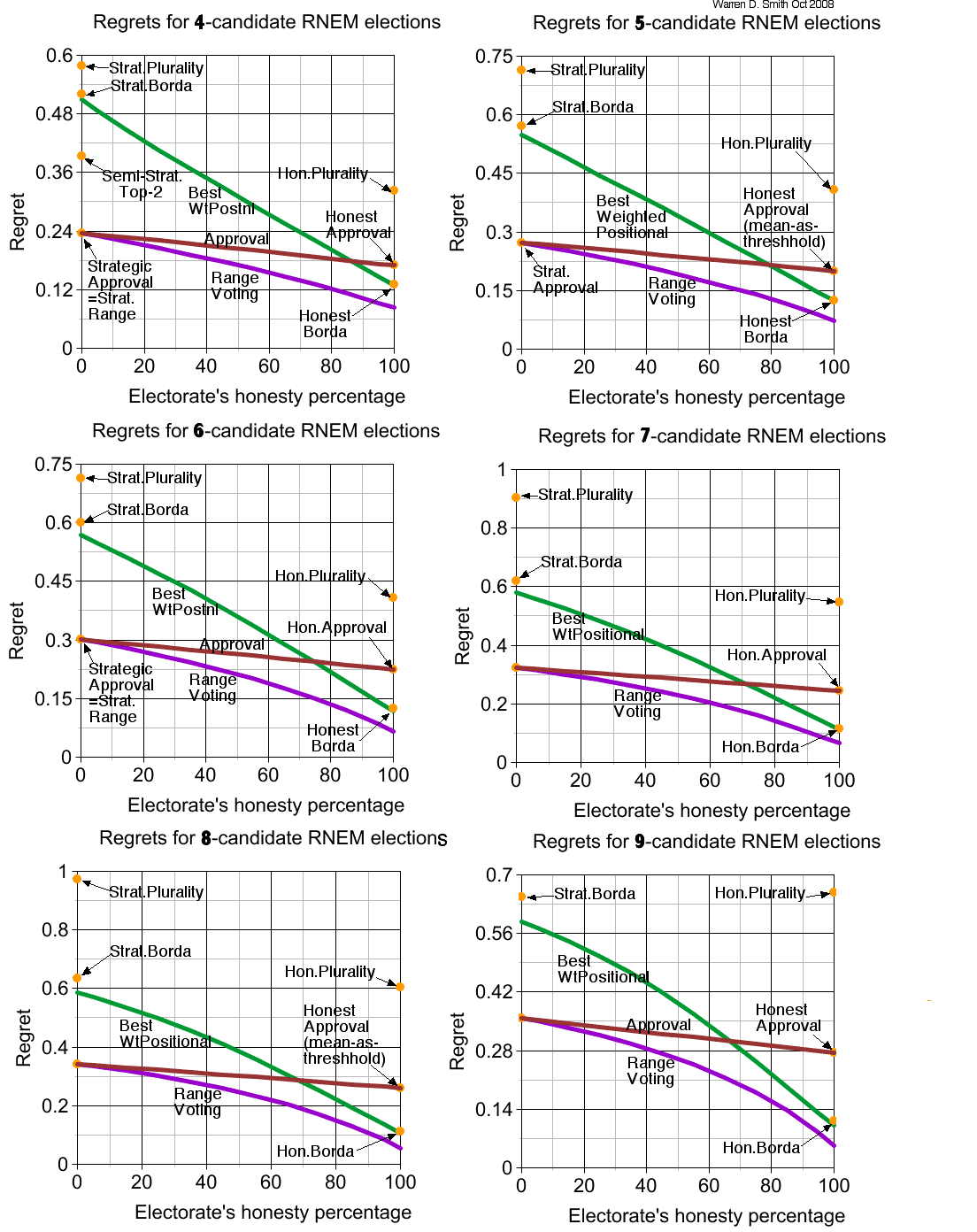
Honest-strategic voter mixtures: Based on that one would guess that when 3≤N≤31 range is superior to the best rank-order voting system for any mixture of H-fraction honest and (1-H)-fraction strategic voters(every H with 0≤H≤100%). Part I had confirmed that guess for N=3 candidates. This paper shall confirm it also for every N with 4≤N≤9, but things get a little trickier. The difficulty is that, with N=3 Part I had shown Borda voting to be a best rank-order voting system, regardless of whether we have honest voters, strategic voters, or any mixture. But when 4≤N the (pseudo)best rank-order voting system depends on H.
Further plans: Section 6 explicitly identifies the pseudo-best rank-order voting system for an honest+strategic voter H-mixture. When 4≤N≤9, it never is Borda for any value of H; but Borda does nearly as well as these best systems especially for small N and high H. Substantially greater regret for Borda versus the pseudo-best rank-order system is only seen (for honest voters) at fairly large N, e.g. N=31.
We then plot regret-versus-H for both range voting and the (pseudo)best rank-order voting system to verify range's superiority at a glance [since the range-regret curve lies below the (pseudo)best-rank-order-curve for every H]. The same numerical methods used to compute table 1 are re-used in constructing these plots. Again, by use of interval arithmetic and rigorous numerical integration, one could in principle mechanically convert all these curve-plots to fully-rigorous proofs, but we have not done so.
Finally, section 7 then considers the limit N→∞ of a large number of candidates, and proves theorems about the asymptotic behavior of the regrets of various voting methods.
If one tries to find the "best" rank-order voting system for moving-average-type strategic voters, one encounters difficulties. The problem is that the voting system can know (or deduce from the strategic ballots with very high probability when V→∞ of making a correct deduction) "God's order." Once it has acquired this knowledge, the voting system can then attempt to compensate for the strategic ballots by acting in an "unfair" way, i.e. by treating different candidates unequally. For example, God's two "frontrunner" candidates, even when ranked first by a voter, presumably would not be given the maximum number of points by the best weighted-positional voting system – and candidates ranked differently by God would be treated differently by the voting system handling any particular ballot. This kind of voting system seems unacceptable in practice because it assumes voters are dishonest/strategic. Well, of course, that was the whole point– but what if some voter actually is honest? In that case the voting system often would artificially re-rank her top-ranked candidate non-top, "refusing to accept" and "altering" her honest vote because "it knows she is lying"! This kind of behavior simply does not seem politically acceptable.
For this reason, it seems better to ask for "pseudo-best" rank-order voting systems. These minimize Bayesian Regret under the assumption that the voters (1) use moving-average strategy, (2) each voter does that under an independent and random notion of what "God's order" is. Pseudo-best voting systems treat all candidates equally.
However, when we actually evaluate BR for a pseudo-best voting system, we shall employ the usual assumption that there is only one "God's order" and all the voters use it as the basis for their strategy. Note that the assumptions used when optimizing the voting system design and the assumptions used when evaluating that design differ. This is the whole point of "pseudobest" versus "best." I admit it is somewhat artificial but I did not see any better way to proceed.
The best versus pseudo-best issue did not arise in Part I because the best and pseudo-best rank-order voting systems in 3-candidate elections are the same (both Borda). However when we have N≥4 candidates as in the present paper, they differ. Section 3 explicitly identifies the pseudo-best rank-order voting system for moving-average-type strategic voters in N-candidate RNEM elections.
More detailed look: The truly best voting system for strategic voters would have a matrix M of weights such that a candidate would receive score Mij if a voter ranked him ith while God's ordering ranked him jth. It would be possible in principle (but we shall not do it) to compute the optimum matrix – in which Mij was the expected utility of the candidate ranked ith by our (assumed strategic) voter and jth by God – and then to compute the Bayesian Regret of the resulting voting system using the correlation-based technology from Part I.
I consider such matrix-voting systems morally unacceptable: the winner ought to depend entirely on the votes and not at all on a priori perceptions from "God" of likelihoods of winning. But even if we were to accept this kind of voting system, we then would encounter a different problem as soon as we tried to use it: how would we decide what "God's order" was to be? The different candidates doubtlessly would argue and sue each other and the election authority endlessly to try to manipulate their position in it.
If we demand that the voting system employ absolutely no information about "God's order" we presumably should have it act as though all God-orderings are exactly equally likely. Unfortunately the voting system, in its quest to optimize societal utility, could try to "outwit" such restrictions by "deducing" God's ordering from the votes themselves, then using the full matrix M. If we forbid that and demand that it really act as though all God-orderings are exactly equally likely, then the optimal (as-restricted) voting system for strategic voters – the pseudo-best voting system – must be a weighted positional system with weights Wi∝∑jMij.
Equivalently, we could simply demand a weighted positional voting system, in which case the best weights for strategic voters (maximizing societal utility) will yield the (genuinely) best weighted positional voting system. So, to summarize the outcome of the preceding argumentation as a "theorem" (albeit that may be a misnomer since it is somewhat in the nature of a "definition"):
THEOREM 1 (PseudoBest Rank Order=Best Weighted Positional): The best weighted positional voting system (i.e. minimizing Bayesian Regret for strategic voters under some model of strategic voter behavior) is the same thing as the pseudo-best rank-order-ballot voting system.
Before the reader dances off into the sunset feeling that the "pseudobest" definition has evaded all problems... there can still be one more problem: With some voter strategic behaviors, the "best" weighted positional system could actually have greater weights for the second-ranked candidate than the top-ranked one! In that case, the voters of course would no longer use that strategic behavior in reality – they'd e.g. switch to ranking their true-favorite "second." The problem here is not that the "best weighted positional" = "pseudobest" definition is wrong; it is that whatever underlying voter strategic behavior model was used, was unrealistic. We shall encounter this exact difficulty in section 3 and propose a cure involving averaging weights in increasing-weight blocks.
We begin by considering a very wide class of voter "strategies" – not just the ones Part I had been considering based on the assumption by voters that everybody besides two known "frontrunner" candidates had negligible winning chances. Instead allow voters to use any function F to determine their votes from candidate-utilities and pre-published information about the candidates and their estimated election chances. Call a voting system fair if it treats all candidates and voters equally, i.e. is symmetric under reordering of either. (Previous authors have called fair voting methods "anonymous and neutral.") We shall only consider fair voting systems in the rest of this paper.
UNDERLYING PRINCIPLE
(optimality of weighted positional under very wide class of voter strategies):
It should be obvious to any reader who has understood the logical flows in
Part I
(see especially its sections 1 and 6)
that the optimum (regret minimizing) fair rank-order voting method in the RNEM with
V→∞ voters is a
weighted positional system in which the weight for the kth-ranked candidate
is the expected utility of that candidate for a random voter
under the RNEM, conditioned
on F producing a rank-ordering ranking him kth.
These weights are just a certain set of constants which can be computed once and for all given
the definition F of voter strategy.
Remark: In consequence, I would expect Approval voting to still provably be superior to every rank-order voting system, for most reasonable strategy notions, for any mixture of honest and strategic voters, in 3-candidate RNEM elections. (However, we are intentionally leaving that somewhat vague; the reader will have to check it for any particular strategy notion.)
We now drop total generality to focus on the moving-average strategy.
Incidental Observation (last-ranked's utility almost irrelevant): In any rank-order-ballot voting system, voters employing the moving-average strategy will produce a rank for God's last-numbered candidate which is, under the RNEM, uncorrelated with and independent of the utility of that candidate (since this vote is determined purely by the utilities of the other N-1 candidates)! More difficulties with correlation matrices will be discussed next section.
A useful sequence Qk: To identify the best fair rank-order voting system for this kind of strategic voter, a useful sequence of quantities to know are Qk, the expected utility of a candidate, conditioned on a voter regarding him as having greater utility than the average-utility of k-1 given other candidates. I.e, Qk is the expected value of a standard normal deviate conditioned on the fact it is greater than the average of k-1 other independent such deviates. If 2≤k this is, as a k-dimensional integral over a halfspace,
where P(x)=(2π)-1/2exp(-x2/2) denotes the standard normal density function. We can evaluate the integral immediately by rotating the coordinate system so that one of the axes becomes perpendicular to the hyperplane
In that case the integrals over all the other k-1 directions can be replaced by just the value at the origin, so the k-dimensional integral becomes 1-dimensional, with value
THEOREM 2 (Best rank-order systems for strategic voters):
For V voters employing the moving-average strategy, the best (i.e. least expected regret) fair
rank-order voting system under the RNEM in the V→∞ limit is, for 2≤N<∞,
the weighted-positional system whose weights are
in decreasing order
SJ(N) for
1≤J≤N.
We have
S1(N)=Q2
while
for 2≤J≤⌊N/2⌋ they are given by this formula
and for J≥⌈N/2⌉ we can get the weights from the negation symmetry
SJ(N)+SN+1-J(N)=0.
Here
binomial(b,a)=b!/[a!·(b-a)!]
where 0!=1.
CAVEAT:
However, when N≥6 these weights SJ(N)
need to be "adjusted" to cure the "disease" that some of them increase with J,
see text below.
REMARK:
The sum-based formula also gives the right answer for S1(N)
provided binomial(a,b) with negative a or b are interpreted in the correct limiting sense.
Proof (of Theorem as supplemented by Caveat):
From linearity of expectations we have that
∑1≤J≤NSJ(N)=0.
From negation symmetry we have
SJ(N)+SN+1-J(N)=0 for 1≤J≤N.
From the first step in the definition of the moving-average strategy, we have
S1(N)=Q2.
Now the remaining weights not yet determined by these relations are
SJ(N)
for
2≤J≤⌊N/2⌋.
For these we argue as follows.
Why would our strategic voter rank a candidate Jth?
If she ranked all except i (i≥0)
of the J-2+i candidates numbered m=3,...,J+i
(where m numbers them in "God's order")
maximum, then also ranked God's (J+i+1)th-numbered candidate
maximum, then that (J+i+1)th-numbered candidate would be ranked Jth in
the voter's strategic rank-ordering and would have expected utility QJ+i+1,
and this event would occur with probability proportional to
It is also possible for Jth rankings to arise
via voters who rank that candidate minimum, in which case
the same formula arises "thinking negated" where the Jth-ranking
from top corresponds to the N+1-Jth ranking from bottom.
Between these we have accounted for every possibility.
(The denominator just comes from normalizing the probability distribution; and since
we may multiply both the numerator and denominator by the same arbitrary constant, we
use that to simplify the exponents in the power of 2.)
This causes the best voting system for strategic voters in 2-candidate RNEM elections to
be weighted positional with weights
We already knew both these facts from
Part I, but for
4-candidate RNEM elections we move into new territory
with the "root3 voting system."
Its weights [rescaled by (3π)1/2] are
Incidentally, note that root3 voting
is the first example (N=4)
where the best weighted-positional voting
systems for honest and for strategic voters differ.
One can now continue on trying
to derive the best rank-order voting systems for strategic RNEM voters
for N-candidate elections for
However, a funny thing happens when N=6 (and presumably for all N≥6):
we find that
S2(N)>S1(N)!
That would mean that a voter would be better off ranking
her favorite frontrunner second rather than first...
contradicting the
validity and whole underlying rationale of
the "best rank-order voting system for strategic voters."
Presumably the right cure for this is to replace any
increasing block of weights by their averages
– albeit when N gets larger
that just leads to further
diseases, see table 2, which require more curing.
With the cures suggested there –
namely that each block of B non-decreasing weights needs to be replaced by B
repetitions of its mean, and this adjustment needs to be re-done until the weights
form a non-increasing sequence –
the resulting voting system will have the property under the RNEM that
a candidate who receives score X from a strategic voter, will, in fact,
then have expected utility X.
(This iterative adjustment process must terminate/converge since each adjustment decreases
the sum of the squares of the weights, hence the process cannot "loop forever.")
That property justifies our claim that the voting system is
"optimal" for this kind of voter – it elects the candidate with the greatest expected
(conditioned on the votes) utility.
QED.
Must "best voting methods for strategic voters" exist?
We have seen that they exist in the RNEM for moving-average strategy with N≥2
candidates and V→∞ voters.
But it is not clear to me that they must exist in general.
The problem is this. Our
"underlying principle"
makes it clear that for any F
defining the strategic behavior, a unique best voting system will exist under
the V→∞ RNEM, but
it might happen that that voting system is such that F no longer
constitutes "sensible strategy." One could, of course, then alter F to make it "more
sensible" and then see what voting system results, and then alter F again, and so on.
The problem is: this
iterative process might enter an infinite loop and never terminate.
So my current answer to this question is "sometimes, but perhaps not always."
More general (albeit perhaps mysterious) remark:
it is well known that there is no such thing as "best strategy"
if one attempts to generalize Von Neumann "game theory" to games with more than 2 players.
So the whole question does not really make sense. "Nash equilibrium" is an attempt to
salvage game theory which often is useful, but for the purposes of voting theorists in
large elections, is extremely useless. [For example,
an election in which every voter votes for the
agreed-by-all-to-be-worst candidate "Hitler," who wins...
is a "Nash equilibrium."]
This explains why we are always focusing on some specific voter behavior F as a strategy
(e.g. the moving-average strategy) instead of enquiring what is
"the best strategy" –
there is no such thing.
| N | Sk(N) for k=1,2,…N (Blocks underlined/italicized) | Block-mean |
|---|---|---|
| 2 | 0.564189583547756, -0.564189583547756 (Plain plurality) | |
| 3 | 0.564189583547756, 0, -0.564189583547756 (Borda) | |
| 4 | 0.564189583547756, 0.325735007935280, -0.325735007935280, -0.564189583547756 (Root3 voting) | |
| 5 | 0.564189583547756, 0.498482082670948, 0, sym | |
| 6 | 0.564189583547756, 0.587688288478586, 0.261953280543306, sym | 0.575938936013171 |
| 7 | 0.564189583547756, 0.633211139753256, 0.442205188900285, 0, sym | 0.598700361650506 |
| 8 | 0.564189583547756, 0.656295438618553, 0.556980936770844, 0.226420506087571, sym | 0.610242511083154 |
| 9 | 0.564189583547756, 0.667957199011994, 0.626712277209905, 0.399505055925336, 0, sym | 0.616073391279875 |
| 31 | 0.564189583547756, 0.679773410167051, 0.721194190473972, 0.741678440464367, 0.753697372447156, 0.761484854452681, 0.766651755249552, 0.769337398026234, 0.767902422857322, 0.757825643105279, 0.730540639763292, 0.673615376561153, 0.573822412896530, 0.423242673970826, 0.225831515802532, 0, sym | 0.728570519141333 |
| 100 | Sk(100) are identical for k=1..39, then decrease for k=40..50. | 0.772901887476515 |
| 316 | Sk(316) are identical for k=1..135, then decrease for k=136..158. | 0.788931905605522 |
NUMERICAL CONFIRMATION: Each line in table 2, for 2≤N≤9, was computed by instead performing 462 million Monte Carlo experiments. (Each experiment was to create N independent standard-normal deviates, compute the moving-average-strategy rank-order vote based on those N utilities, and keep track of the mean utility of the candidate ranked Jth in these votes for each J with 1≤J≤N. The thus-obtained Monte-Carlo results, rounded to 4 decimal places, were found to agree with the exact SJ(N) formula in every case to within an error of ±1 in the final decimal place.
Part I had already given closed formulas for the correlation matrices for, e.g, every honest weighted-positional rank-order voting system. We now give a few more (without proof; in most cases the proofs are easy – or at least easy consequences of integrals tabulated in appendix B of Part I – but in other cases the computation is more difficult)
For 4-candidate semi-strategic "top 2" voting, the "C-matrix" (explained in Part I) can be computed in closed form. It is "doubly rank-deficient"
    [ 0.5642 -0.5642  0.0000  0.0000  0.6028  0.0000 ]
C ≈ [-0.5642  0.5642  0.0000  0.0000 -0.6028  0.0000 ]
    [ 0.0000  0.0000  0.5642 -0.5642  0.0000  0.6028 ]
    [ 0.0000  0.0000 -0.5642  0.5642  0.0000 -0.6028 ]
where the exact formulas for the numbers given as decimals are
0.5642≈π-1/2 and
0.6028≈(1-2/π)1/2.
We have
      [ 1 -1  0  0 ]
CCT = [-1  1  0  0 ]
      [ 0  0  1 -1 ]
      [ 0  0 -1  1 ]
and all vote-variances are 1.
THEOREM 3 (Best Semi-Strategic Rank-Order=Top-2): The best (regret-minimizing) semi-strategic voting system, under the RNEM with V→∞ voters, in 4-candidate elections, is "top-2" voting, i.e. the weighted positional system with weights proportional to (+1, +1, -1, -1).
Proof: By our underlying principle from section 2, it has to be weighted positional with weights proportional to expected utilities (in the eyes of any given voter) conditioned on that voter's vote. Because of our postulate/definition that "God" chooses the two frontrunners (and two non-frontrunners) randomly in a way unrelated to all voters' utilities, and because of our definition of "semi-strategic" voting, the two frontrunners and two non-frontrunners are exactly symmetric, so their weights must be the same, and by translation and scaling we can make them be (+1,-1). QED.
For 4-candidate Strategic Approval=Range we have rank-deficiency 1 and
    [ 0.5642 -0.5642  0.0000  0.0000  0.6028  0.0000  0.0000 ]
C ≈ [-0.5642  0.5642  0.0000  0.0000 -0.6028  0.0000  0.0000 ]
    [-0.3257 -0.3257  0.6515  0.0000  0.0000  0.6028  0.0000 ]
    [-0.2303 -0.2303 -0.2303  0.6910  0.0000  0.0000  0.6028 ]
      [ 1 -1  0  0 ]
CCT = [-1  1  0  0 ]
      [ 0  0  1  0 ]
      [ 0  0  0  1 ]
All vote-variances are 1, and the additional exact formulas are
    [ 0.5642 -0.5642  0.0000  0.0000  0.0000  0.6028  0.0000  0.0000  0.0000 ]
C ≈ [-0.5642  0.5642  0.0000  0.0000  0.0000 -0.6028  0.0000  0.0000  0.0000 ]
    [-0.3257 -0.3257  0.6515  0.0000  0.0000  0.0000  0.6028  0.0000  0.0000 ]
    [-0.2303 -0.2303 -0.2303  0.6910  0.0000  0.0000  0.0000  0.6028  0.0000 ]
    [-0.1785 -0.1784 -0.1784 -0.1784  0.7136  0.0000 -0.0001  0.0000  0.6028 ]
      [ 1 -1  0  0  0 ]
      [-1  1  0  0  0 ]
CCT = [ 0  0  1  0  0 ]
      [ 0  0  0  1  0 ]
      [ 0  0  0  0  1 ]
All vote-variances are 1, and the additional exact formulas are
0.1784≈(10π)-1/2 and
0.7136≈(5π/8)-1/2.
REMARK: Note that in all the cases above, det(CCT)=0 so that the vote-vote correlation matrix CCT is not positive-definite; it is merely semidefinite. A zero-eigenvalue eigenvector is (1,1,0,...,0), but this is not bothersome since strategic voters always vote (x,-x) in the first two coordinates and hence never "activate" this eigenvector.
A much more annoying indefiniteness problem occurs with 5-candidate psubest-strategic-rank-order voting,
      [ 1.0000 -1.0000  0.0000  0.0000  0.0000 ]
      [-1.0000  1.0000  0.0000  0.0000  0.0000 ]
CCT = [ 0.0000  0.0000  1.0000 -0.7071 -0.7071 ]
      [ 0.0000  0.0000 -0.7071  1.0000  0.0000 ]
      [ 0.0000  0.0000 -0.7071  0.0000  1.0000 ]
where the exact formula for 0.7071 is 2-1/2.
This also has det(CCT)=0, arising from the unique eigenvector with
zero eigenvalue, which is Experiments with the Monte-Carlo code showed, however, that
This same problem arose in other cases too, but the same fix has always worked in our experience so far.
Alan Gibbard, in his proof of his version of the Gibbard-Satterthwaite theorem, focused attention on the following two randomized voting methods, which, he showed, were the unique two "strategy-proof" rank-order voting systems (and probabilistic mixtures of these two):
THEOREM 4: Under the RNEM with V→∞ voters, "random ballot" has the same regret as "random winner." Also, "random pair" has the same regret as "strategic plurality voting."
Proof: is immediate from the definition of the RNEM and our model of strategic plurality voting. QED.
In the real world, our model of the two "frontrunners" being "selected randomly by God" is not completely correct. I suspect, indeed, that the two frontrunners have better quality on average than random candidates. (But this certainly is not always the case. For example, two US presidents often selected by historians as the "worst" are George W. Bush and Warren G. Harding. It is hard to believe that their respective third-party opponents Ralph Nader and Eugene V. Debs would have made worse presidents than them. Debs was actually a political prisoner at the time of the election but Harding, once elected, pardoned him.) If so, then random pair in the real world presumably would have worse regret than strategic plurality voting.
THEOREM 5 (Best rank-order system for honest+strat voter mix): The pseudo-best rank-order voting system in N-candidate elections in the V→∞ voter RNEM with a mixture of H-fraction honest and (1-H)-fraction strategic, voters, is weighted positional with weights
The proof is immediate from the underlying principle from section 3.
With the optimum voting system known, we then can employ the known methodology from section 8 of Part I to evaluate its Bayesian regret for an H:1-H honest+strategic voter mixture. When I did so using our usual numerical-integration-based "correlation-based procedure," the result was the following plots. The other curve plotted is the regret for range voting using the same H:1-H voter mixture – the strategic range voters are using moving-average strategy and thus are effectively using approval voting.
Interesting aside: The best rank-order system is only a little better than Borda when N∈{4,5}.
As you can see immediately from the plots (and the case N=3 is covered in Part I)
CLAIM: Range voting is superior to every rank-order voting system (even the best) in the V→∞ voter RNEM, for N-candidate elections with 3≤N≤9, at any voter-honesty fraction H with 0≤H≤100%, provided we ignore the distinction between best and pseudobest. (That is, more precisely: the regret of range voting is less than the regret of the pseudo-best rank-order system at every H, where the "pseudo-best" system minimizes regret in a model where the strategic voters each have independent uniform-random beliefs about "God's likelihood order," but then actual regret is evaluated in a setting where there is only one, publicly known, such order.)
What about 7, 8, 9,..., candidate elections? It would be nice to have a theorem proclaiming range voting's superiority versus the best rank-order system for every number N≥3 of candidates. That is a good question. It is often possible to prove ∫A(x)dx>∫B(x)dx despite the absence of closed formulas for either integral. We know what the best rank-order system is for honest voters (see Part I's section 6) and we know the pseudo-best system for strategic voters (here) so that we know what "A(x)" and "B(x)" are; the difficulty is that our integrals are multidimensional. An interesting task for future authors, then, would be to develop suitable "comparison theorems" enabling such proofs.
Since I currently lack such tools, it is useful to consider the limit of N→∞ candidates. The idea is that if we can show something for both N≤31 and for N→∞, that makes it plausible that it works for all N.
THEOREM 6 (Range voting's regret is small for large #candidates): For honest range voting in the RNEM with V voters, V→∞, as the number of candidates N becomes large, the regret is O(1/lnN)1/2 times the regret of "random winner."
Proof sketch: Use the results about the variances associated with the Gk(N) in Part I's appendix A to see that all the "normalization factors" for range voters will be equal up to relative error O(1/lnN) (except for an arbitrarily small fraction of voters, which hence will have an arbitrarily small effect on total utilities). We can now use, e.g, Chebyshev's bound on probability densities with bounded variance and more strongly, Hall's work cited in that appendix showing exponential tail bounds; and also we can use the fact that all voters are independent and have independent utility-versus-range-vote errors, combined with the Chernoff bound, to see that, with probability→1, all the range-vote totals will be the same as the corresponding true-utility-totals, up to additive errors whose root mean square has order ±V1/2(lnN)-1/2. Meanwhile the maximum among the N true utility totals will almost surely be of order V1/2(lnN)+1/2. Thus (now again using facts about the Gk(N) from Part I's appendix A) even the maximum among the errors in approximation of utilities by vote totals will still be far smaller – by a factor of order (lnN)1/2 at least – than the maximum utility, QED.
In contrast,
THEOREM 7 (Other regrets are large for large #candidates): For each of these weighted positional voting systems: plurality, antiPlurality, Borda, and median-as-threshold approval voting (or, indeed, any weighted positional system in which at least a positive constant fraction of the system-defining weights differ by at least a positive constant fraction of full scale from the optimum weights given in Part I's section 6) in the RNEM with V honest voters, V→∞, as the number of candidates N becomes large, the regret tends to a positive constant times the regret of "random winner."
Proof sketch: Each vote will, as an approximation to utility, have additive |error| (on average for each voter) a constant fraction of full scale. All these errors are independent, leading via the central limit theorem when V→∞ to the vote totals having an expected additive |errors| (as an approximation to summed candidate-utilities) of order V1/2, which (note) is the same typical order as the |utilities| themselves and all these errors are independent in the V→∞ limit. Therefore, if we elect the candidate with maximum vote rather than maximum utility, we will lose utility (i.e. experience regret) of the same order as the maximum utility. QED.
REMARK: I conjecture that the pseudo-best rank-order system (for V→∞ strategic voters under the RNEM) has the same order regret as strategic approval voting and random winner, but with a better constant factor than random winner. This would follow immediately if we could prove that at least a positive constant fraction of the SJ(N) are equal, as empirically appears to be the case, for large N.
REMARK: I conjecture that the best rank-order system (for V→∞ honest voters under the RNEM) has the same order regret as range voting but with a greater constant factor due to its effective artificial uniformization of the intercandidate utility spacings. It easily may be shown that Borda, median-as-threshhold Approval, and Plurality have successively worse constant factors in their regrets in the large-N limit. I also conjecture that strategic approval voting also obeys theorem 7 and with a strictly better constant factor than random winner.
THEOREM 8 (Strategic and Mean-based "honest" Approval asymptotically same): Strategic (moving-average strategy) and honest (mean-based threshhold) have with probability→1 asymptotically the same regrets in the RNEM with V honest voters, V→∞, as the number of candidates N becomes large.
Proof sketch: The idea is that the moving average is essentially the same as the full average (both converge to 0 under the RNEM) for almost all of the N candidates, when N→∞. Hence the approximations of utility-totals by vote-totals will have asymptotically the same distributions for both voting methods. QED.
THEOREM 9 (Strategic Plurality for large #candidates): For strategic plurality voting, in the RNEM with V honest voters, V→∞, as the number of candidates N becomes large, the regret is asymptotic to the regret of random winner. (This is also true for the "random ballot" election method.)
Proof:
Consequence of our exact regret formulas and
Part I's appendix A –
in its notation the expected regret of
strategic plurality is
Another question is: "what about other statistical/political models besides RNEM (such as D-dimensional politics models, etc)?" Can future authors prove analogous results to ours in those models? With the help of some fortuitous miracles we are able to accomplish that in some cases. That will be explained in a new paper "part III."
References:
G.Alefeld & J.Herzberger: Introduction to Interval Computations, Academic Press, 1983.
Alan Gibbard: Manipulation of Schemes that Mix Voting with Chance, Econometrica 41 (1977) 587-600.
R. Hammer, M. Hocks, U. Kulisch, D. Ratz: Numerical Toolbox for Verified Computing I: With Algorithms and Pascal-XSC Programs, Springer-Verlag, Berlin, 1994.
Eldon Hansen & G. William Walster: Global Optimization using Interval Analysis (2nd ed.) Marcel Dekker, New York, 2004.
Nicholas J. Higham: Computing the nearest correlation matrix – a problem from finance, IMA Journal of Numerical Analysis 22,3 (2002) 329-343; also "A Preconditioned Newton Algorithm for the Nearest Correlation Matrix," 2008 preprint available herehttp://eprints.ma.man.ac.uk/1086/01/covered/MIMS_ep2008_50.pdf.
Ramon E. Moore: Interval Analysis, Prentice Hall, Englewood Cliffs, N.J., 1966.
Ramon E. Moore: Methods and Applications of Interval Analysis, SIAM, Philadelphia PA 1979.
Miodrag S. & Ljiljana D. Petkovic: Complex Interval Arithmetic and Its Applications. Berlin: Wiley, 1998.
Page summarizing all 3 papers in this series