By Warren D. Smith, warren.wds AT gmail.com, Nov-Dec. 2014.
Suppose you perform N independent statistical tests. One fails with p-level a. Another fails with p-level b. ... Another fails with p-level z. What is the probability of this combined event? Call the answer FN(a,b,c,...,z). This seems an innocent question, but as we shall see, answering it in full leads to an astonishing smorgasbord of combinatorial mathematics, eventually culminating when we find an algorithm for computing it in O(N2) steps while storing O(N) numbers. Also important is the function PN(a,b,c,...,z) which gives the p-value associated with F, i.e. would be its cumulative distribution function if F's N arguments were i.i.d. random numbers uniform in [0,1]. This whole paper can be viewed as a study of these two functions. Why are these questions important? Because they are central to the meaning and usefulness of "statistical significance." If we do not know how to combine different statistical significance (p-level) values, especially in the easiest case when they are for independent tests, then we don't know how to do much. And yet, in spite of the logical centrality of these questions, they appear to be new. This all is one "MCP effect" (Multiple Comparisons Problem in statistics). At the end, we discuss MCP and support Ioannidis' claim that the majority of published scientific research findings are wrong.
We may assume wlog (without loss of generality) that 0≤a≤b≤c≤...≤z≤1 (sortedness) because otherwise, the correct answer is obtained by sorting the N arguments into increasing order and then applying the formula that is valid under the pre-sortedness assumption. Note that any function that is computed by the following 2-step procedure
Extended definition: Although the domain 0≤a≤b≤c≤...≤z≤1 is adequate for all purposes in statistics, it sometimes is useful to allow the larger domain a≤b≤c≤...≤z, which we accomplish by tacitly agreeing that if any of these arguments are greater than 1, then they are automatically "clipped," i.e. replaced by 1; and if any are less than 0, they too are clipped by replacement by 0. Also, besides allowing all integers N≥1, it also can be useful to define F0()≡1.
F1(a)=a, of course. It is not the case that F2(a,b)=ab. Actually,
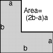
Because: that is the chance that if x and y are independent uniform(0,1) randoms, then either x<a and y<b, or x<b and y<a. I.e, exactly as I said in the problem statement, word for word, this is "the chance that one test fails with p-level a and another with p-level b." See figure for this subregion of the square 0<x<1, 0<y<1 in the xy-plane. Please make sure you appreciate this. I gave the written problem description to 5 competent mathematicians in a row, and, incredibly, not one came up with the right formula for F2(a,b), so there is something funny about this problem causing many people to find it very confusing/deceptive. It is probably my fault for wording it in some funny bad way(?). If I had worded it as "the chronologically first test fails with the lesser p-level a and the second with the greater p-level b," then the correct answer would have been ab. However that would be the answer to a different problem, one that is not the subject of this paper. The "or" tells us that the answer to our problem, generally is greater than ab. Indeed, F2(a,b)>ab if and only if b>a>0.
In that area argument, x (and y) are the CDFs of whatever function is being evaluated by the first (and second) statistical test. Any (continuous) CDF of any random variable, automatically is a uniform(0,1) random variable. If x<p, then that is the definition of "failing the test with p-level p."
Fundamental definitions: A statistical test is a procedure that inputs some data and/or makes some experimental observations, and outputs a function of it, p, which is a real number in the interval [0,1] which, if the "null hypothesis" about that data/observations were true, would be random and uniformly distributed. (Note. Some people may have other conventions about the output of a statistical test. Whatever their output is, it is a random variable R, and the CDF, under the null hypothesis, of R can be regarded as our "p." Thus, regardless of what other stupid conventions anybody else may have, if their CDFs are continuous you can always convert them to our uniform-in-[0,1] convention.) If this output p is very small, such as p=0.001, or large, p=0.999, then the statistical test is said to fail with p-value p. Such failures indicate the null hypothesis is probably false, and p tells you how confident to be about that assertion. We can (and generally will) restrict our attention to low failures (i.e. p≤0.001) because we can define q=2min(p,1-p) and then regard q as the p-value of a different statistical test; and the new test fails low if and only if the original test failed either high or low. Then statistical significance for us shall mean "the p-value" where smaller p means we are more confident the null hypothesis is false; confidence shall mean 1-p.
Our whole "combining p-values" statistics problem arises all the time in real life. Here are some examples.
Example #1: Fairness of coin.
I want to convince you that your coin is biased towards heads.
I tell you: "I performed two tests on your coin.
Each consisted of tossing it 10 times and counting the number of heads that arose.
The set of test results was {6,7}."
How convinced should you be that your coin is unfair? You note that the exact probability
a truly-fair coin would produce ≥6 heads in 10 tosses, is b=193/512,
and the chance it would produce ≥7 is a=11/64. You therefore conclude
Illuminating counterexample for coin fairness (Charles Greathouse): The null hypothesis is that it's a fair coin. My test 1 consists of flipping the coin twice and seeing if both times it comes up heads; p=1/4. Test 2 consists of flipping it once and seeing if it comes up heads; p=1/2. The chance that a fair coin would fail both tests is 1/8, not F2(1/4,1/2)=3/16.
What went wrong here is that Greathouse's two tests were not interchangeable (unlike in the first coin-testing example), or – to delineate the cause more precisely – it is because Greathouse provided us with "extra information." That is, in this case, from Greathouse's description of his two tests and the p-value set {1/4,1/2}, we know that the 1/4 had to be the result of test 1, since it is impossible for test 2 to produce a p-value 1/4. Therefore, in this case, we know that the p-values x and y of tests 1 & 2 had to be (1/4,1/2) in that order and cannot have been (1/2,1/4). This allows us to deduce the combined p-value 1/8, which is the area of the rectangle
If, however, Greathouse had only told us "I performed two tests on your coin, and one had p-value 1/4 and the other 1/2" without providing that extra information, then all we would be able to deduce would have been p=3/16, the area of the L-shaped region
Example #2: How amazing is it that the last 5 US presidents have been tall?
|
|
An answer is F5(0.022, 0.064, 0.075, 0.126, 0.244)≈6.071×10⁻⁵. I.e. if you'd picked 5 random people and determined their heights, the chance that their 5 height p-values (among age&sex cohort), after sorting, would lie in the intervals [0,0.022], [0,0.064], [0,0.075], [0,0.126], [0,0.244] would be 6.071×10⁻⁵. If we'd only asked about the last two presidents BHO & GWB, then F2(0.126, 0.244)≈0.0456. If we'd asked about the last 10 presidents, F10(0.005, 0.022, 0.064, 0.075, 0.126, 0.157, 0.209, 0.244, 0.244, 0.523)=4.0×10⁻⁷.
Example #3: Sanity check.
Some people seem convinced that
FN(a,b,c,...,z)=abc...z.
That is not true; the right hand side actually is only a lower bound.
If you think this equality holds, you will get extremely wrong answers.
As a sanity check, I suggest that you compute the product of 100 independent
random uniform(0,1) numbers. I just did that 22 times. The products I got all lay
between 2×10-52 and
2×10-35.
That's obviously far too small.
In contrast, for example,
Just to try to make that ultra-clear: The 100 numbers Hj are p-levels for the event "a random uniform is chosen, and turns out to be ≤H." The total event here is of course not remarkably improbable – it happens all the time that 100 numbers are ≤themselves, and is not at all a sign something must be wrong with the random number source. But since ∏1≤j≤100Hj is very tiny this constitutes a high-confidence contradiction if you'd wrongly thought F100=∏1≤j≤100Hj.
Example #4: Monte-Carlo check. It appears empirically that the expectation value of F5(B,C,D,E,1) when A,B,C,D,E are five i.i.d. uniform(0,1) random variates after sorting into order A<B<C<D<E, is about 0.524, but the expected value of BCDE is about 0.127. If you are one of those thickheaded people who still think F5(B,C,D,E,1)=BCDE, then I strongly suggest that you perform this Monte Carlo computation yourself to prove the disagreement. You do not need any formula for F5 to do so. All you need is a source of random-uniform numbers, the ability to test whether x<y (and hence to sort), and be able to count – each time we generate 10 i.i.d. uniform(0,1) random numbers a,b,c,d,e,A,B,C,D,E, a "success" is the event that
Equivalently, a "success" is the event that
I then laboriously recalculated those Monte-Carlo approximate values exactly via 5-dimensional symbolic integration (using the F5 formula we shall present below), getting 11/21≈0.52381 as the exact "success" probability, and 8/63≈0.12698 as the exact expected wrong answer, respectively.
I apologize for the over-long and over-many examples. All I can say is, it has been proven by test that many otherwise competent people will not believe this if fewer examples are stated.
What are the formulas for F3(a,b,c), F4(a,b,c,d), and so on? It is possible to determine these by working out certain N-dimensional volumes via something like an inclusion-exclusion argument; FN(a,b,c,...,z) is the volume of the region
where there are N! parenthesized clauses, one for each permutation of the N coordinates xj. Each of these N coordinates may be regarded as an independent uniform(0,1) random variable, representing the CDF of whatever random variable is being tested by one of the tests. Each of the clauses represents an N-dimensional "brick" hyperrectangular region, so the OR of all the N! clauses is the union of N! such hyperrectangles. But this volume computation gets more and more painful. Indeed, a straightforward evaluation of the volume of this union via inclusion-exclusion would be a sum of 2N!-1 terms. Note the factorial inside the exponent. This is infeasible if N≥5.
But we shall devise more efficient methods. With our first, exactly evaluating FN with N=40 should be achievable on a single computer. With our second method, N=80 should be feasible. Our final method should enable reaching N=106. (Here "exactly" means, more precisely, "up to limitations imposed by roundoff error in machine arithmetic." Our algorithms would produce exact results if there were no roundoff error.)
As easy lower and upper bounds,
Both these bounds can be tight: When a=b=c=...=z=ζ it is easy to exactly work out the special case
in which the lower bound is tight. And the upper bound is tight in the limit
as is trivial to see in the volume picture because in this limit
the overlaps all have relatively negligible volume.
Where between these two bounds does the truth usually lie?
Some of our results later suggest there is a sense in which, very roughly, "usually,"
Another trivial bound is
Scaling lemma: FN(γa,γb,γc,...,γz) = γN FN(a,b,c,...,z) for any scaling factor γ with 0≤γ≤1/z. (Trivial consequence of the N-dimensional volume problem formulation.)
Fundamental Recurrence Theorem: The following recurrence provides the exact answer in general:
This holds because if ζ is the random variable [from among a set of N+1 independent uniform(0,1) random variables; i.e. the CDFs of the N test outputs] that happens to be minimal, then it must obey 0<ζ<a while the N others must satisfy the conditions for FN rescaled from the interval [a,1] to [0,1].
By using the F-recurrence I compute these exact formulas:
Monotonicity Corollary: if 0<a<b<c<...<z<1 then the partial derivative of FN(a,b,c,...,z) with respect to any of its arguments always is positive. This is trivially true for N=1 and N=2, and then is trivially proven by induction on N via the Recurrence (although it seems not obvious at all if you do not know the recurrence!).
2nd-Derivative Corollary: if 0<a<b<c<...<z<1 then the second partial derivative of FN(a,b,c,...,z) with respect to any of its N arguments always is non-positive. (Indeed, it always is negative, except it if it was the last, i.e. maximum, argument, in which case it is 0 because F is always a linear function of its final argument if the others are regarded as fixed.) This again is trivially true for N=1 and N=2, and then is trivially proven by induction on N via the Recurrence (realizing as a lemma that the function [b-ζ]/[1-ζ] of ζ is decreasing and concave-∩ for all ζ with 0≤ζ≤1 given that 0≤b≤1).
Mixed Partials Corollary: if 0<a<b<c<...<z<1 then the partial derivative of FN(a,b,c,...,z) with respect to any two of its N arguments (N≥2), for example ∂b∂cFN(a,b,c,...,z), is always positive. (Same proof.)
Sensitivity bound I: if 0<a<b<c<...<z<1 then the partial derivative of FN(a,b,c,...,z) with respect to any of its arguments (call the argument we are considering "x") always is upper bounded by NFN/x.
Proof: Let S=1+δ/x with δ>0.. Then FN(a,b,c,...,x+δ,...,z) < FN(aS,bS,cS,...,xS,...,zS) = FN(a,b,c,...,x...,z)SN by monotonicity and the scaling lemma. Now subtract FN(a,b,c,...,x,...,z) from both sides, divide by δ, and then take the limit as δ→0. Q.E.D.
Sensitivity bound II: if 0<a<b<c<...<z<1 then if the N arguments of FN(a,b,c,...,z) are changed to values at most a multiplicative factor (1+ε) away from their original values, then the value of F changes by at most a multiplicative factor of (1+ε)N.
Expectation-value Theorem: If EN is the expectation value of FN(a,b,c,...,z) when a,b,c,...,z all are independent uniform(0,1) random variates after sorting into order, then EN=1/(N+1). Equivalently, given two N-tuples (a,b,c,...,z) and (A,B,C,...,Z) of i.i.d. random real numbers drawn from the uniform(0,1) density, the chance the first N-tuple (after sorting) is less than the second N-tuple (also after sorting) in every coordinate – "vector domination" a<A, b<B, ..., z<Z – exactly equals 1/(N+1).
Proof (Gareth McCaughan): Put all 2N numbers together and sort them. Now go through them in order and move North 1 unit when you see a lowercase letter and East one unit when you see a CAPITAL letter. (Start at the origin x=y=0.) The vector domination criterion is the same as saying that you never go below the diagonal line x=y. The fact that you chose N of each says that you end up at (N,N).
But now we have a familiar problem with a familiar answer. The number of grid-paths with this property is the same as the number of properly-nested sequences of 2N parentheses containing N "(" and N ")": the Nth Catalan number. And, as every schoolchild knows, that equals Binomial(2N,N)/(N+1). This is indeed 1/(N+1) times the total number of (not-necessarily balanced) parentheses-sequences. Q.E.D.
Remarks about this kind of theorem & proof: Many people find this answer EN=1/(N+1) to be surprisingly large. (My first guess was that the answer was 2-N.) McCaughan's "put 'em all together; sort; North & East" trick essentially converts our continuous kind of problem into a discrete Bertrand ballot type problem.
Bertrand's classic ballot problem: Let k be a positive integer. (For us, and in Bertrand's original publication, k=1.) Suppose that candidates A and B are in an election. A receives a votes and B receives b votes, a≥kb. What is the probability that throughout the counting of the ballots in chronological order, A's total always exceeds k times B's total? Answer:(a-kb)/(a+b).
Whitworth's version of the problem (which we use): What is the probability that throughout the counting of the ballots in chronological order, A's total always is greater than or equal to k times B's total? Answer when k=1:(a+1-b)/(a+1).
This is called "Bertrand's ballot problem" since it was originally posed and solved by W.A.Whitworth in 1878. (See Barton & Mallows 1965. J.L.F.Bertrand rediscovered it in 1887. The generalization allowing arbitrary integer k≥1 was discovered by E.Barbier in 1887 and proven by J.Aebly in 1923.) One famous solution method is the "Andre reflection method," so-called because it was not the method used by D.Andre in his 1887 solution. A variant of that method by Goulden & Serrano 2003 is published, along with some history, in Renault 2007. It also is possible to solve all these problems with the aid of the cyclic lemma: "For any m with 1≤m≤N: if a1,a2,...,aN is a sequence of integers with ∑jaj=1, then there is exactly one cyclic shift of this sequence having exactly m positive partial sums" – and/or the more general version of that lemma given by Dershowitz & Zaks 1990. They also give references showing it too has been rediscovered a large number of times. Also, a more general theorem than ours, with a proof very similar to McCaughan's, was given by Feller in §III.9 of his probability theory book, concerning "Galton's rank order test." This was so called because in 1876 Francis Galton deduced a totally unjustified conclusion from some data of Ch.Darwin because he did not understand that, due to our theorem, the vector domination probability is much larger than he suspected. His name was then immortalized in honor of his stupid error.
Vector Domination-Order Theorem: Given K random real N-tuples (A(j),B(j),C(j),...,Z(j)) for each j=1,2,3,...,K, with all entries drawn independently from the uniform(0,1) density, the chance that each N-tuple (after sorting) is greater than all its successors (also after sorting) in every coordinate – "total order by vector domination" – exactly equals
Proof: The simplest way to prove it is to invoke the famous Frame-Robinson-Thrall hook length formula to count the orderings of the NK numbers which are compatible with the demands [as a subset of the (NK)! total orderings]; and then divide by the total number (NK)!/N!K of ways to place NK numbers in an N across by K down array so that each row is ordered. Q.E.D.
A more general problem was already solved on page 175 of MacMahon 1909 (see also page 160 for the Whitworth/Bertrand special case). It also is possible to prove it by: Put all KN numbers together and sort them. Now scan through them in order regarding a number arising from a tuple of type J as a "vote" for candidate J in an election. The multiple vector domination criterion is equivalent to the Jth candidate remaining ahead, or tied, with the Kth, whenever J<K, throughout the counting of the ballots as they arrive in the scan order. (Each candidate has exactly N votes in all.) Equivalently, we count lattice paths in the K-dimensional integer lattice which go from (0,0,0,...,0) to (N,N,N,...,N) via NK unit steps in such a way that every point (y1,y2,...,yK) of the path is in sorted descending order (equalities permitted). Without demanding sortedness, the total number of such lattice paths would be the "central multinomial coefficient" (KN)!/N!K. With the demand, this counting problem was solved by Zeilberger 1983.
Vector Multiple-Domination Problem: Given K random real N-tuples (A(j),B(j),C(j),...,Z(j)) for each j=1,2,3,...,K, as well as another (a,b,c,...,z) with all entries drawn independently from the uniform(0,1) density, what is the chance that (a,b,c,...z) (after sorting) is greater than all K other N-tuples (also after sorting) in every coordinate: a>A(j), b>B(j), ..., z>Z(j) for each j=1,2,...,K?
Answer when K=2 (double domination):
Proof: This (by the argument soon to follow) is equivalent to the fact that the number of 3N-step lattice walks from (0,0,0) to (N,N,N), containing only integer points (x,y,z) having x≥y and x≥z, equals
The argument: Put all (K+1)N numbers together and sort them. Now scan through them in order regarding a number arising from a tuple of type J as a "vote" for rival J of a given candidate in an election. The multiple vector domination criterion is equivalent to our given candidate remaining ahead of, or tied with, every one of his K rivals, throughout the counting of the ballots as they arrive in the scan order. (Each candidate has exactly N votes in all.) Equivalently, we count lattice paths in the (K+1)-dimensional integer lattice which go from (0,0,0,...,0) to (N,N,N,...,N) via (K+1)N unit steps in such a way that every point (x,y1,y2,...,yK) of the path obeys x≥yj for each and every j=1,2,3,...,K. Without demanding the first coordinate be maximal, the total number of such lattice paths would be ([K+1]N)!/N!K+1.
Now for general K≥3, I have no idea what the walk-count is. But, by a miracle, when K=2 we have a nice simple formula for it. This formula already arose as the solution A006335 of a two-dimensional lattice-path-counting problem, called "Kreweras walks"! See the unobtainable Kreweras 1965, and the highly obtainable Bousquet-Melou 2005, for 101-page and 41-page long proofs of Kreweras's miraculous counting formula. To solve our problem of counting certain 3-dimensional lattice paths, we now need to explain why our problem is equivalent to Kreweras's counting problem for certain closed-loop 2-dimensional lattice paths.
In our 3D walk problem, consider 2D cross-sections arising from cutting planes of form x+y+z=T where T is integer valued time. The three allowed steps (1,0,0), (0,1,0) and (0,0,1) project in the 2D cross section to 3 different directions 120° apart. In each 2D cross section, we really have got a point set which is the vertices of the usual tessellation of the plane by equilateral triangles, and then we step from a vertex to one of an allowed set of 3 among its 6 neighbors as time advances by 1, then re-step, and so on. The walk ending at (N,N,N) after 3N timesteps is equivalent in the 2D projection to "walks which return to start point." The 3D demands x≥y and x≥z are equivalent in the 2D projection to staying always within a fixed 120° wedge whose corner is the start-point. Now if we apply a linear transformation to this equilateral triangle lattice to distort the 3 allowed step directions to become (-1,0), (0,-1), and (1,1) in the XY plane, whereupon the vertex set becomes the integer lattice (tessellation of the plane using unit squares), and the allowed wedge becomes the quadrant X≥0, Y≥0. This converts us into the Kreweras walk problem described by Bousquet-Melou 2005 on her first page. That proves our 3D lattice walk problem is bijectively equivalent to her (and Kreweras') 2D walk problem, explaining why our count formula is the same. Q.E.D.
Variance Theorem: If VN is the variance of FN(a,b,c,...,z) when a,b,c,...,z all are independent uniform(0,1) random variates after sorting into order, then
Proof: The answer to the vector double-domination problem is the expected value of FN(a,b,c,...,z)2; and then use the formula var(X)=E(X2)-E(X)2 and the expectation value theorem. (The asymptotic result at far right valid when N→∞ comes from Stirling's formula.) Q.E.D.
Long side remark about Kreweras and Gessel's "miraculous walk-counting formulas": Gessel & Zeilberger 1992 solved the problem of counting "lattice walks that stay within Weyl chambers of arbitrary Coxeter reflection groups." (See also Grabiner & Magyar 1993.) Their idea was to use the "Andre reflection method" which is a combinatorial analogue of Kelvin's method of image charges in electrostatics. That was very nice, but if the region the walk is restricted to, is not a Weyl chamber of a Coxeter reflection group, then it gives us nothing. Now in what seemed to be an almost inexplicable miracle, Kreweras 1965 discovered his counting formula for a certain particular kind of restricted lattice walk. And Ira Gessel in 2001 discovered another such miracle, which seemed even more inexplicable.
Our 3D formulation of Gessel's problem: Count the 2N-step walks on the FCC lattice starting at (0,0,0) and ending at (0,0,2N) with allowed steps being to nearest neighbors. Note, the FCC (face centered cubic) lattice consists of all integer 3-tuples (x,y,z) with x+y+z even. Gessel also imposes the demand that all the walk points (x,y,z) must stay in the region x≥0 and x+y≥0 defining a 135° wedge.
Gessel's walk-counting formula was finally proven by Kauers, Koutschan, Zeilberger 2009 using very heavy computerized algebra (estimated to involve formulas about 250 pages long).
One of KKZ's equivalent 2D formulations of Gessel's problem: The number of ways of walking 2N steps in the region x+y≥0, y≥0 of the square-lattice with unit steps in the east, west, north, and south directions, that start and end at the origin x=y=0, equals 16N K [Γ(5/6+N) Γ(1/2+N)] / [Γ(5/3+N) Γ(2+N)] where K=[Γ(5/3)Γ(2)]/[Γ(5/6)Γ(1/2)].
KKZ conjectured computer assistance was necessary, i.e. felt it was impossible for unaided humans to prove Gessel's counting formula. Eventually, though, a (still rather long) "human proof" was found, by Bostan, Kurkova, Raschel 2014.
We now point out that there may be a simple unified explanation both the Kreweras and Gessel "miracles." However, after some discussion with Alin Bostan and Ira Gessel, it appears that my explanation is most likely only partial. The new idea is simply the old Gessel-Zeilberger 1992 "walks in Weyl chambers / Andre reflection" idea, except that there are a few more Coxeter groups than they'd thought. This is because, for lattice walks in two dimensions only, we can consider the underlying space to be, not the Cartesian XY plane, but rather the Riemann surface of zw, i.e. featuring integer winding number w around the origin z=0 in the complex z plane. With this greater scope, we can now define Coxeter reflection groups as usual using "mirror lines" that pass through the origin. We then get a "Coxeter group" in any case where the angle θ between two rotationally-consecutive lines obeys
If, further, reflection about a line with angle θ to the X-axis happens to be a symmetry of the underlying lattice – for the square lattice this means θ is a multiple of 45°, and for the equilateral triangle lattice it means θ is a multiple of 30° – then the whole Gessel-Zeilberger method using Andre's reflection trick goes through perfectly happily if we are trying to count lattice walks that stay within an angle-θ wedge. If θ happens to be a divisor of 360° with even quotient, then we do not get a "miracle" but rather an "expected event using the old Gessel-Zeilberger thinking"; only in other cases do we need a Coxeter group that G&Z had not already known about. The complete table of predicted alleged miracles, then, will be:
| # | Lattice | θ | H | Counts of walks that start & end at origin (0,0) | Notes |
|---|---|---|---|---|---|
| 1 | △ | 120° | 1 | 1, 0, 3, 4, 26, 80, 387, 1596, 7518, 34656, 167310, 813384, 4040212, 20285408, 103195235, 530042604, 2748206006, 14362312640, 75609109594, 400620871608, 2135307326508, 11442213676512, 61615122713550, 333282537518040, 1810222600024044, 9869776566646080, 54002852920884540, 296449512451881360, 1632343645230788520 | A151372 |
| 2 | △ | 150° | 1 | 1, 0, 3, 4, 27, 84, 419, 1756, 8473, 39752, 195760, 968104, 4892378, 24957278, 128936196, 671983900, 3533365192, 18714554170, 99796938574, 535352099024, 2887534929785, 15651152169808, 85215057908750, 465873973561938, 2556583654159437, 14078689046794064, 77778973017819575, 430981498786694326, 2394755129231075218 | ? |
| 3 | △ | 120° | 2 | 1, 2, 16, 192, 2816, 46592, 835584, 15876096, 315031552, 6466437120, 136383037440, 2941129850880, 64614360416256, 1442028424527872, 32619677465182208, 746569714888605696, 17262927525017812992 | Kreweras |
| 4 | △ | 150° | 2 | 1, 2, 17, 216, 3330, 57545, 1072326, 21082108, 431406658, 9106370280, 197047243752, 4351014294393, 97708108984581, 2225656274729522, 51319743620874018 | ? |
| 5 | ▢ | 135° | 1 | 1, 2, 11, 85, 782, 8004, 88044, 1020162, 12294260, 152787976, 1946310467, 25302036071, 334560525538, 4488007049900, 60955295750460, 836838395382645, 11597595644244186, 162074575606984788, 2281839419729917410, 32340239369121304038, 461109219391987625316, 6610306991283738684600 | Gessel |
In this table, H=1 if every step from a node to its nearest neighbor is allowed, but H=2 if only the even numbered ones (counting anticlockwise starting from the X-axis direction as "zero") are allowed. In the H=2 cases, returning walks necessarily are 3N steps long (and for ▢ necessarily 2N); but in the other cases any integer N≥0 is allowed as the number of steps. Further, we expect full understanding of the walk counts can be obtained for every θ that is a multiple of 30° in the △ case, and every θ that is a multiple of 45° in the ▢ case (among θ≤180°, plus we could also allow the no-wedge case θ=360°). However in many of these cases neither we, nor anybody else, has actually carried through the Gessel-Zeilberger 1992 formalism to obtain the understanding that we predict is available for the taking. Furthermore, the "Green function" for any "multiply wound lattice graph" will depend on the starting point (unlike for plain lattice graphs, which are translation-invariant) and it often is far from obvious what it is. But in all the ▢ cases, and all the △ H=2 cases except when the wedge angle is 150°, walk-count formulas are already known:
| θ | Count for 2N-step ▢ walks | Asymptotic |
|---|---|---|
| 0° | (2N)!/(N![N+1]!) | 4NN-3/2π-1/2 |
| 45° | 6(2N)!(2N+2)!/(N![N+1]![N+2]![N+3]!) | 16NN-524/π |
| 90° | (2N)!(2N+2)!/(N![N+1]!2[N+2]!) | 16NN-34/π |
| 135° | Gessel, W0=1, (N+2)(3N+5)WN+1=4(2N+1)(6N+5)WN | 16NN-7/322/3Γ(1/3)/(3π) |
| 180° | (2N)!(2N+1)!/(N![N+1]!)2 | 16NN-22/π |
| (360°) | (2N)!2/N!4 | 16NN-1/π |
| θ | Count for 3N-step △ walks (H=2) | Asymptotic | Conjectured asymptotic for N-step △ walks (H=1) |
|---|---|---|---|
| 30° | δN0 | 0 | 6NN-7C30, C30≈2197.93223512621 |
| 60° | 2(3N)!/(N![N+1]![N+2]!) | 27NN-431/2/π | 6NN-4C60, C60≈14.885880176374 |
| 90° | (3N)!/(N!2[N+1]![2N+1]) | 27NN-331/2/(4π) | 6NN-3C90, C90≈1.3295531906286 |
| 120° | Kreweras 4N(3N)!/([N+1]![2N+1]!) | 27NN-5/22(3/π)1/2/4 | 6NN-5/2C120, C120≈1.2694265629813 |
| 150° | ? | 27NN-11/5K150, K150≈0.1670193739 | 6NN-11/5C150, C150≈0.65041301862 |
| 180° | (3N)!/(N!3[N+1]) | 27NN-231/2/(2π) | 6NN-2C180, C180≈0.8269933431319 |
| (360°) | (3N)!/N!3 | 27NN-131/2/(2π) | 6NN-131/2/(2π), see A002898 |
Ries (number-guessing program by Robert Munafo) points out that
The numerical C values should be precise except perhaps for the last two decimal places given, albeit the C150 and K150 values may have less accuracy because they seemed exceptionally difficult for my Richardson-extrapolation method.
Alin Bostan comments: "All of the tabulated conjectures (except for the values of the constants C) may be proven using Denisov & Wachtel 2012 and many examples of that approach may be found in Bostan, Raschel, Salvy 2014. Your guessed values for C60 and C120 both are correct as may be proven using the known generating functions for these sequences (A151366 and A151372) which are
respectively. Here C60 will be shown in forthcoming work by A. Bostan, F. Chyzak, M. Kauers, L. Pech, and M. van Hoeij; and C120 is comparatively easy to show since for it the generating function is algebraic. It is also possible to determine C180 in a similar way: First one should prove that the sequence WN of walk-counts obeys the recurrence
with initial values W0, ..., W14 = 1, 0, 4, 6, 42, 140, 720, 3150, 15610, 75432, 380016, 1921920, 9901584, 51438816, 270160176 (we have a general result that arbitrary walks in the half-plane have D-finite generating functions); then with aid of software by Mark van Hoeij and his student Vijay Kunwar we find that its generating function is
then finally the asymptotics of WN may be deduced using singularity analysis. For C90 I first numerically confirmed your conjectured value to 23 decimal places, then found a 5th-order recurrence, which was solved by van Hoeij to find the generating function
agreeing with A057648, which again ought to yield a proof for C90. The cases θ=150° and θ=30° very probably do not have D-finite generating functions in which case their constants C are not deducible using our current techniques."
Summary: we've pointed out a common feature of the Gessel and Kreweras "miracles" which also might seem to predict 3 additional "miracles." I then conducted tests seeking recurrence relations obeyed by these 3 additional sequences; then Alin Bostan did a much more extensive search, with neither of us finding any (although our searches both easily found the recurrences obeyed by Kreweras and Gessel). Consequently Bostan conjectures none of the other three return-to-0 walk-count "predicted miracle" sequences are "D-finite." The whole connection we have explained to Coxeter reflections may nevertheless be useful (even in the absence of exact formulas) for, e.g. determining asymptotics. The self-returning walk count always is asymptotic to BNN-AC where B depends only on the valency within the lattice step-graph in an obvious way, A depends only on the wedge angle θ and not on the lattice-step-graph – specifically A=1+180°/θ if 0<θ<360° – and the C's are nonnegative constants. It might be that our connection is a necessary, but not sufficient, ingredient for the existence of such "miracles." Bostan, Bousquet-Melou, and their numerous collaborators have between them got a large number of automated techniques and associated theory for finding (and often proving) recurrences and generating functions arising in 2-dimensional restricted lattice-walk-counting problems, which as you can see have immense power. In particular I doubt any human unaided by computers, even Ramanujan, could have found the generating functions Bostan et al gave just above. If our Coxeter-connection can be exploited that would be an additional weapon. It also is noteworthy (and as yet unexplained, but presumably it arises from the reflection method) that the constants for θ=180° happen, in all three tabulated cases, to be equal to the constants for θ=360° times small integers (2, 1, and 3). (End of long side remark.)
What about the third moment of F, namely, Expectation(F3)? This arises similarly from the solution of the vector triple-dominance problem, which arises from solving a 4D lattice-walk-counting problem, namely finding the count W3(N) of 4N-step walks on the integer lattice Z4 from (0,0,0,0) to (N,N,N,N) which obey t≥max(x,y,z) always. The W3(N) count-sequence begins
for N=0,1,2,...,15,
and
[all vector entries are ±1 with even number of minus signs, these 4 are the vertices of an origin-centered regular tetrahedron; this walk takes place on the "BCC lattice" (Body-centered cubic)] and the restriction is: the walk remains confined within the closed octant-like trihedral cone, (but with all three dihedral angles equal to 120°, not 90°) defined by
Only one initial step is possible, (+1,+1,+1). On the second step, all 4 are possible.
Comment by Alin Bostan: "The above sequence 1, 6, 288, 24444,... is exactly the 3D Kreweras-like sequence we mentioned in Figure 4 (page 18) of Bostan, Bousquet-Melou, Kauers, Melczer 2014! Specifically, we counted 4N-step walks on the integer lattice Z3 starting at, and returning to, (0,0,0), subject to the constraint that they always remain within the non-negative octant min(x,y,z)≥0. Our set of allowed steps was
Although we computed the first 5000 terms with a supercomputer, our software was unable to recognize any recurrence, hence we suspect it is not D-finite. We numerically found the asymptotic behavior 0.0977·256N/N3.32585, which is the same as your asymptotic provided your exponent 1.83 is, more precisely, 1.82585, and your constant 0.8 is, more precisely, 0.769. My belief was this exponent was an irrational number, which if so would prove the sequence is not D-finite." Ries points out that (5/φ)1/4+2=3.32585365756... where φ=(1+√5)/2≈1.61803 is the golden ratio.
The fourth moment Expectation(F4) similarly arises from the solution of the vector quadruple-dominance problem, which arises from solving a 5D lattice-walk-counting problem, namely counting 5N-step walks on the integer lattice Z5 from (0,0,0,0,0) to (N,N,N,N,N) which obey t≥max(w,x,y,z) always. This also can be rephrased as 4D self-returning lattice-walk-counting problems, e.g. 5N-step walks starting and ending at (0,0,0,0), staying in the non-negative orthant, and with steps
The W4(N) count-sequence begins
for N=0,1,2,...,13, and
Other expectation values: The harmonic mean of FN(a,b,c,...,z) is 0 for each N≥1, just because ∫0<a<1da/a=∞ and FN(a,b,c,...,z)≤min(a,b,c,...,z)=a.
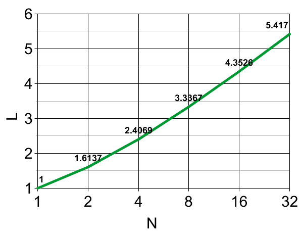
If LN denotes the expectation of |lnFN(a,b,c,...,z)| when the N arguments are uniform random in (0,1) after sorting, then L1=1, and L2=3-ln(4)≈1.613705638880109; but L3≈2.0582 probably cannot be expressed in closed form, at least without using polylogarithmic functions.
The lower bound is from Jensen's inequality using the concave-∩ nature of the ln(u) function, combined with the known expectation value 1/[N+1] of FN. The upper bound is simply because FN(a,b,c,...,z)≥abc...z combined with the fact that L1=1 and using linearity of expectations. The table and plot below (computed using Monte Carlo integration) suggest that the lower bound is closer to the truth, and indeed perhaps LN∼1.6lnN≈1.1log2(N) when N→∞.
| N | LN |
|---|---|
| 1 | 1 |
| 2 | 1.6137 |
| 3 | 2.0582 |
| 4 | 2.4069 |
| 5 | 2.6938 |
| 6 | 2.9377 |
| 7 | 3.1493 |
| 8 | 3.3367 |
| 9 | 3.5045 |
| 10 | 3.6564 |
| 11 | 3.7956 |
| 12 | 3.9235 |
| 16 | 4.3526 |
| 24 | 4.9718 |
| 32 | 5.417 |
| 48 | 6.05 |
| 64 | 6.5 |
Median:
Empirically, when 7≤N≤50 the median MN
of the distribution of FN
when its N arguments are i.i.d. uniform(0,1) random numbers after sorting, obeys
Returning to the plain expectation value 1/(N+1) of FN, it tells us a number of interesting things. Based on it, it would seem that to truly assess statistical significance we need to use ([N+1]/2)FN, not FN, and not (even worse) abc...z. Pay attention – many common errors are being refuted here. The ([N+1]/2) factor can be thought of as approximately compensating for the fact there are many possible test-describing N-parameter sets the inviligator could have chosen, and if he "cherrypicks" exactly the toughest such test by choosing a,b,c,...,z after having seen the data to be tested beforehand, that makes said data look artificially bad. (This whole phenomenon basically does not happen if N=1, it is only a multi-test effect.)
So returning to our presidential-heights example, I of course had cherrypicked
exactly the toughest such test, by using exactly the sorted-set of the five
p-values themselves, as the test parameters.
The answer corrected for
the cherrypicking-of-tests effect via the factor (N+1)/2=3 is
Example #5: Wars and religion. How amazing is it that the 6 wars that started between 2000-2014 ("war" defined as having more than 10000 fatalities) tended to involve comparatively religious countries?
| # | Countries | War | Dates | Fatalities | %irreligious | p |
|---|---|---|---|---|---|---|
| 1 | Syria | Syrian civil war | 2011-2014 | ≥43K | 15 | 0.536 |
| 2 | Pakistan | NW Pakistan war | 2007-2014 | ≥23K | 4 | 0.175 |
| 3 | Congo+Rwanda | Kivu conflict | 2006-2013 | 10K | 5 & 5 | 0.221 |
| 4 | Iraq+Syria | IS "caliphate" | 2014 | ≥9K and rising | 15 & 15 | 0.536 |
| 5 | Iraq v. USA | Iraq war & insurgency | 2003-2013 | 29-600K | 15 v. 36 | 0.630 |
| 6 | Afghanistan v. USA | Afghan war | 2001-2013 | 54K | 3 v. 36 | 0.597 |
It's a bit hard to answer this question since it depends on exactly what the definitions of "war" and "religion" are, and for each particular war, which countries we claim were involved. For example, in the case of the Afghanistan/USA war, it could be argued that there were 2 or 3 subwars going on. I'll define the "percentage of irreligious population" in a country according to the definition used by Gallup polls (their data 2006-2011). For each war, I'll define Q to be the unweighted average of the two (or one) participating country's irreligion-percentages (ignoring third, fourth, etc countries that may have participated to comparatively minor extents), and the associated p-level to be the fraction (among the 154 Gallup-polled countries) of countries with smaller irreligion-percentage than Q, plus half the fraction with equal. (Actually, this unweighted average Q is arguably the wrong quantity to use, but that only can matter for wars 5 & 6 and in those two cases all reasonable rival quantities still yield almost the same p-levels, so it does not matter much.) I find F6(0.175, 0.221, 0.536, 0.536, 0.597, 0.630)=0.040. This would naively be thought 96% significant, but before rushing to the journals to publish this finding, consider that multiplying that p-level by the cherrypicking correction factor 3.5 yields 0.140. If only the first 4 wars, i.e. the ones not between two opposed countries, are considered, then F4(0.175, 0.221, 0.536, 0.536)=0.044 which cherrypick-corrects to 2.5F=0.109.
Example #6: what happens if this cherrypicking correction is not employed? If it is not, then you will be easily fooled. For example, suppose you have a perfectly fair coin. I claim "Your coin actually is highly nonrandom." As proof of this, we toss your coin 100 times. I now tell you "on toss 1, the result was heads, a p=1/2 event. On toss 2, it was tails, a p=1/2 event. On toss 3, tails, a p=1/2 event. Etc. The combined p-value for the combined event was F100(1/2,1/2,...,1/2)=2-100 which proves your coin is extremely nonrandom. Incidentally, I did not tell you while we were performing the experiment, but I correctly predicted every single one of your coin tosses." Utter nonsense. Similarly, I will be able to convince you that any long sequence of random events proves incredibly huge nonrandomness, if I have the freedom to lie, post-experiment, about what my 100 "predictions" were. (This in fact was exactly what was done by famous Ponzi-scheme con artist Bernie Madoff, who would publish 'records' of the stock trades supposedly made for his stock fund by his 'advanced proprietary algorithm'; these lists of trades were in fact constructed by Madoff afterwards and made his algorithm appear amazingly successful.)
For that particular coins problem, the appropriate "cherrypicking correction factor" would be 2N-1 to compensate for the ability of Madoff to choose one of 2 directions each coin flip. But for our problem assuming arbitrary p-levels within the real interval [0,1] are possible, and if we do not allow the freedom to choose directions each time, it is (N+1)/2.
As another example,
suppose I want to "prove" elections in the 50 US states were "fraudulent."
I simply point out that every one of the 50 observed
election margins being larger than one would have expected
from its pre-election (or exit) polls
was an event with some p-value, and then note that F50
of those 50 p-values is some extremely small number.
If you are gullible, will be forced to believe me.
The way not to be gullible is to apply the cherrypicking
correction and enquire about the value of
If you were even more gullible and wrongly believed FN(a,b,c,...,z)=abc...z, then you would be even easier to convince of "fraud" because the con-artist would have an extra factor of up to N! at his disposal, i.e. here the factor would be up to 25.5×50!≈7.7556×1065, rather than a mere factor of (N+1)/2=25.5. And in fact, the "ElectionIntegrity" email group contains people who have in the past done exactly this. They (1) do not use the cherrypicking correction, (2) do not use the correct FN formula, but rather the incorrrect product formula (because, as one of them, Joshua Mitteldorf, explained to me in email, that is "the standard formula"), and then (3) claim – outrage!!! – that they have "proven" by multiplying various p-values together that, with super-huge confidence, various elections were fraudulent. In fact, it is their analysis that was fraudulent. [Mind you, the elections they had in mind, might also have indeed been fraudulent! I am merely pointing out that the confidence numbers coming from their analyses were bunk.] I have now examined several "scientific papers" posted by members of that group (including Mitteldorf) before Nov. 2014. Every one contained exactly this so-called methodology and stated no awareness/mention whatever of either (1) or (2) – nor indeed, of the entire "multiple comparisons problem" in statistics. When I attempted to point this out by posting to that email group, I was immediately censored by its moderator Michael B. Green, who refused to allow my refutation to be posted there.
General-purpose con: In any situation with somebody trying to convince you of something where the convincer gets to choose her tests after seeing the N data, a gullible person will be vulnerable to these cons, but if they know the exact FN formula and know about the (N+1)/2 cherrypicking correction factor – or 2N(N+1)/2-factor, in the bidirectional case – then they will not be.
Isn't this "cherrypicking correction factor" an inexact kludge? Yes. And a rather crude one, too.
So what is the correct thing to do? PN: Define
Also define
Example #7: Improving TestU01 suite for random number generators. TestU01 is a freeware ANSI C software library for empirical statistical testing of uniform random number generators. For example, according to their user guide, their "SmallCrush" battery consists of 10 statistical tests of randomness; their "BigCrush" battery applies 106 tests. Each outputs a p-level, which – if the random number generator being tested were truly random uniform – would be an independent uniform(0,1) real number. At the completion of any SmallCrush run, it prints a summary telling you all the "suspicious" tests, i.e. the ones whose p-level outputs lay outside the interval [0.001, 0.999]. For example, it might report that the "BirthdaySpacings" and "MaxOft" tests failed with p-levels 0.00017 and 0.999934 respectively. The user's guide tells you not to worry too much about a test failure at the p=0.001 level because with hundreds of tests one would be reasonably likely to fail at that level even with true random numbers. Fortunately (?) BigCrush can usually be depended on to massacre most alleged random generators with p≤0.0000000001 or p≥0.999999999 level failures. But assuming we've found a generator that survives BigCrush without any massively-obvious test failures – then what? I suggest that it would be better if SmallCrush, BigCrush, etc were to add the following to their summary:
This final output then truly would be a summary of the net conclusion of the whole battery of tests, and if it reported that p<0.001, then your generator is probably a failure, despite (perhaps) every individual test result from that battery being OK!
Comment by Pierre l'Ecuyer: Two difficulties:
I now determine the exact formulas for the first two PN's.
First, P1(a)=a is trivial.
It is harder to work out
P2(a,b).
Because
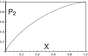
Doing the three integrals, we find
As checks, note that when X∈{0,1} this expression correctly yields X. If integrated dX from X=0 to 1, we get 2/3, confirming our previous claim the expectation value is 2/(N+1), here with N=2. The X-derivative of P2, which can be regarded as a probability density on (0,1] rather than a CDF, is
which is indeed always non-negative when 0<X≤1.
This density is everywhere decreasing, since its derivative
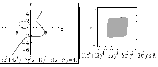
To explain the futility of continuing on: If we were now to try to work out P3 we would need to compute the volume of a subset of the unit cube bounded by several algebraic surfaces of degrees up to 3. In general, PN is the volume of a subset of the unit N-cube bounded by multiple algebraic surfaces of degrees up to N. Although it might be possible to do a few more, in general, it is impossible to express such quantities in closed form. Indeed, as has been known from the time of Abel and Galois, it is not even possible to solve polynomial equations of degree≥5 in closed form. Hence for example the area of a rectangle defined by sextic(x)quadratic(y)≥0, where the sextic has exactly two real roots, usually is not expressible in closed form. For an explicit impossibility conjecture, consider the finite-area loop containing (-2,1) bounded by the pictured cubic curve
I doubt this area can be expressed in closed form, at least without employing general elliptic functions. (It was computed by numerical integration.) And if we ask for the area inside any reasonably general quartic curve such as
then I doubt even that elliptic functions suffice.
Incidentally,
Nevertheless, there are useful statements we can make about the PN when N≥3.
"Density exhibits Logarithmic-Infinity" Theorem: For all sufficiently small X, for any fixed N≥2, PN(X) is bounded between two positive constants times X|ln(X)|+X.
This is because
(bounded by a generalized hyperboloid)
is of order
"Density exhibits Power-Law Zero" Theorem: Define the Nth harmonic number Harm(N)=1+1/2+1/3+...+1/N. Then for all sufficiently small ε>0, for any fixed N≥2, 1-PN(1-ε) is bounded between two positive constants times εHarm(N).
Proof sketch. In this argument we shall always be assuming ε>0 is sufficiently small and that k and K denote constants (whch can depend upon N and may vary in different uses) with 0<k<K. The argument for N=4 is:
but
It should be obvious how this generalizes to handle arbitrary N≥2. The second set of inequalities can be "seen geometrically" in the N-volume picture by realizing that certain hyperrectangles within the unit N-cube [0,1]N and touching the (1,1,1,...,1) corner are empty, e.g. a 1×1×1×(1-d) slab, or a 1×1×(d-c)×(d-c) one, and so on. The first set of inequalities is since, contrarywise, no such hyperrectangle is empty. Q.E.D.
As a result of these theorems, it would seem that there ought to be good approximations to ProbDensN(X)≡∂XPN(X) of the form
("good" meaning "with uniformly bounded relative error, which can be made arbitrarily small by increasing K") provided the constants A,B,C,D,...,J are chosen to be the right functions of N. For example, with K=2 we could choose A,B,C so that the first three moments
assume their correct (exactly known) values
This can be accomplished in closed form by using the "Euler Beta" integral
and (which is obtained by differentiating with respect to α)
The resulting expressions for A,B,C unfortunately are about a page long, even though
they can be simplified using
where γ≈0.5772156649 is the Euler-Mascheroni constant. One can go further in the same way, also using the 3rd and 4th moments to determine D and E too. Here are the results. (Note the minus signs on B and D, convenient because it makes the tabulated numbers usually come out positive.) Of course there is no need for the N=1 and N=2 lines of this table since we have exact formulas for PN when N=1 and N=2. Those lines are included purely to enable comparing our approximation with the exact formula: when N=1 our approximation is exact, when N=2 it is accurate to about 1%. If a root X exists in (0,1) at which the probability density crosses 0 then, since negative probabilities are disallowed, we conclude that our approximation is insane. This apparently happens exactly when N≥13. (Presumably sanity could be restored by using more moments and coefficients, but we have not tried.) Another possible symptom of insanity is if the probability density has an extremum at some X with 0<X<1, i.e. does not merely monotonically decrease. This first happens when N=10 (extrema at X≈0.76 & 0.84); for 1≤N≤9 our approximate probability densities each are monotone decreasing.
| N | A, –B, C, –D, E; root X |
|---|---|
| 1 | A=0, B=1, C=0, D=0, E=0; no root |
| 2 | A=22/45, B=(110880ln2+8389)/113400, C=143/336, |D|=1859/6720, E=2431/24192; no root |
| 2 | A≈0.488888888888889, B≈0.75172098219124, C≈0.425595238095238, |D|≈0.276636904761905, E≈0.1004877645502645; no root |
| 3 | A≈1.329755802325247, |B|≈0.9899990091517885, C≈4.132151773926948, |D|≈4.026518217119707, E≈1.769533977685182; no root |
| 4 | A≈2.309689075329896, |B|≈3.529838559851989, C≈10.32257860536279, |D|≈10.99563018190612, E≈5.041713051631158; no root |
| 5 | A≈3.322782715261376, |B|≈6.435344596459465, C≈18.05441231789685, |D|≈20.34882035099093, E≈9.620714279349611; no root |
| 6 | A≈4.320109811684, |B|≈9.472388022191717, C≈26.66325358153077, |D|≈31.33793481198389, E≈15.18518377395709; no root |
| 7 | A≈5.279945280532916, |B|≈12.51649435687646, C≈35.72151155746683, |D|≈43.40316962216263, E≈21.46788611467915; no root |
| 8 | A≈6.19362892512384, |B|≈15.50208562976144, C≈44.95963858595925, |D|≈56.14606057029857, E≈28.2629690808137; no root |
| 9 | A≈7.058862456790246, |B|≈18.39563259388122, C≈54.20851884329598, |D|≈69.28685485962319, E≈35.41581308070953; no root |
| 10 | A≈7.876438563069318, |B|≈21.18135839547317, C≈63.36254948558761, |D|≈82.6295231722304, E≈42.81106945066427; no root |
| 12 | A≈9.378193259951761, |B|≈26.4116544458683, C≈81.15162794853983, |D|≈109.4112928858642, E≈58.00615000728443; no root |
| 13 | A≈10.068246457727, |B|≈28.8588699846163, C≈89.7255075592614, |D|≈122.686138326376, E≈65.6931676418314; X≈0.6531 & 0.7370 |
| 24 | A≈15.767389194826, |B|≈49.921727859668, C≈169.30439740855, |D|≈255.42636011583, E≈147.04922657127; X≈0.5249 & 0.7536 |
Examining the exact FN formulas for N=2,3,4,5,6,7, they evidently keep getting messier. Various attempts to re-express them in simpler ways by, e.g. replacing arguments x by 1-x, or F by 1-F, or seeking polynomial factorizations, all failed. One perceives a few patterns easily proven by induction on N, such as: FN is always an N-variate homogeneous polynomial of degree=N with integer coefficients; the polynomial degree with respect to the Kth argument (regarding all the others as fixed) is N+1-K for each K=1,2,3,...,N; the sum of the coefficients equals 1; the coefficient of aN is always (-1)N-1; and the coefficient of abc...z is always +N!. But those facts, while nice, fall well short of a complete understanding.
Aha! Beautiful conjectural full answer: After fiddling with F3-F7 to rewrite them with their terms in "standard order" (as presented above – rightmost expressions), and F2(a,b)=[-a+2b]a, I saw that the (unsigned) coefficients are exactly the "multinomial coefficients for compositions in standard order," see A124774; the exponent vector on each monomial term encodes the composition. A "composition of N" is an ordered sequence of positive integers whose sum is N. There are exactly 2N-1 compositions of N, hence the expression for FN has exactly 2N-1 monomial terms. What is the encoding and what are the signs? There is a natural sign associated with each composition of N as follows. (I'm not sure anybody ever realized this before – it is the composition analogue of both the well known concept of the sign of a permutation and the even-better known concept of the "parity of a binary word.") Begin with the composition N=1+1+1+...+1, encoded by the monomial abc...z=a1b1c1...z1 which we declare always has positive sign. View this as 1 ball in box#1, 1 ball in box #2,... 1 ball in box #N. Now move balls from one box to another, one at a time, until reaching the desired monomial. For example, starting from a1b1c1d1 we can reach a2b0c1d1 via one move. If m is the minimum number of balls that need to move (all moves leftward!) needed, then the sign of that monomial is (-1)m. To explain the encoding, the monomials in F5 correspond to the compositions of 5 in standard order via
| a5 | ab4 | a2c3 | abc3 | a3d2 | ab2d2 | a2cd2 | abcd2 | a4e | ab3e | a2c2e | abc2e | a3de | ab2de | a2cde | abcde |
| 5 | 4+1 | 3+2 | 3+1+1 | 2+3 | 2+2+1 | 2+1+2 | 2+1+1+1 | 1+4 | 1+3+1 | 1+2+2 | 1+2+1+1 | 1+1+3 | 1+1+2+1 | 1+1+1+2 | 1+1+1+1+1 |
and the monomials in F4 correspond to the compositions of 4 in standard order via
| monomials | a4 | ab3 | a2c2 | abc2 | a3d | ab2d | a2cd | abcd |
|---|---|---|---|---|---|---|---|---|
| compositions | 4 | 3+1 | 2+2 | 2+1+1 | 1+3 | 1+2+1 | 1+1+2 | 1+1+1+1 |
| binary words | 111 | 110 | 101 | 100 | 011 | 010 | 001 | 000 |
| signs | – | + | + | – | + | – | – | + |
My point is that it also is possible (bijectively equivalently, although this equivalence may not have been previously known) to define a "composition of N" to be an eligible ordered sequence of exactly N nonnegative integers summing to N – the degree-vector of each of our monomials – where the ball-moves it takes to reach an eligible monomial starting from a1b1c1...z1 always are leftward moves (and this defines what it means for a monomial to be "eligible"). The bijection between these two definitions of the composition concept is illustrated for N=4 and N=5 in the tables above.
I have also added 3rd and 4th rows to the table for N=4 to also show the (previously known) bijection between the 2N-1 compositions of N and the (N-1)-bit binary words; and showing the sign of each composition. This also illustrates another way to compute the sign: it is (-1)w where w is the number of 1-bits in the binary word. This bijection-to-binary is explained in this picture stolen from wikipedia:
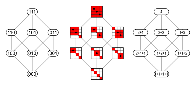
(see also MacMahon 1893) and one can also biject directly from binary-word to monomials because the 1-bits in the binary word (read from left to right) encode the "missing letters" in the monomial in reverse-alphabetical order.
The multinomial coefficients for the compositions of 5 are
5 4+1 3+2 3+1+1 2+3 2+2+1 2+1+2 2+1+1+1 1+4 1+3+1 1+2+2 1+2+1+1 1+1+3 1+1+2+1 1+1+1+2 1+1+1+1+1
1  5  10   20   10   30    30    60      5   20    30     60     20     60      60      120
because 1=5!/5!, 5=5!/(4!1!), 10=5!/(3!2!), 20=5!/(3!1!1!), etc.
Summary of answer: The formula for FN(a,b,c,...,z) is a polynomial in its N arguments of homogeneous degree N, having exactly 2N-1 monomial terms. There is a 1-to-1 correspondence (described above) between the "compositions of N" and these monomial terms. Each monomial is divisible by a. The unsigned coefficient of each term equals the multinomial coefficient for its composition, which always is an integer. Its sign is the sign (described above) naturally associated with that composition.
And hence, as corollaries, the unique maximum |coefficient| equals N!, its sign always is +, and it multiples the monomial abc...z; and the unique minimum |coefficient| always is (-1)N-1, multiplying the monomial aN.
The sum AN of the |coefficients| is given by A000670, the "Fubini numbers." The sum of the signed coefficients of course equals 1 since FN(1,1,1,...,1)=1. The sum BN of the squared coefficients is, for N=0,1,2,3,...,
which agrees, at least up to here, with the sequence A102221. If this agreement continues, then from the generating function by Vladeta Jovovic claimed there,
we deduce that BN is asymptotic to N!2C/KN where K≈0.8171226656316 is the positive solution of BesselI0(2√x)=2, and C≈0.83357.
The main result of this paper is: that answer is correct! We will not be able to prove it until later.
A more general question which is easily answered once our initial question is answered, is this. Suppose among N random quantities, some M exist which fail some statistical test with the M different p-levels a,b,c,...,z where 0≤a≤b≤c≤...≤z≤1. What is the p-level for this combined event? The answer is
And for this more general question, the appropriate "cherrypicking correction factor" would be (M+1)/2 by McCaughan's same proof as above.
Trying to understand the FN can become quite addictive. E.g,
Arithmetic Sequence Theorem:
This can be proven by induction on N by using the recurrence. Indeed, more generally, one can in the same way evaluate F of the arithmetic sequence equispaced from Q to 1
for any given Q with 0<Q<1, where Δ=(1-Q)/(N-1). And of course a fully arbitrary arithmetic progression (not necessarily with endpoint 1) can be handled by applying the Scaling Lemma to this result, yielding
Harder is the
Geometric Sequence Theorem:
and this pattern presumably keeps going. "The pattern"?
Well, the coefficients are (-1)N times those in the "list partition transform"
A133314; the exponents on the leftmost (factored out) term
arise from the "triangle number" sequence
         The 5 partitions of 4:    4 =   3+1 =   2+2 =   2+1+1 =   1+1+1+1
   The corresponding exponents:    6   3=3+0   2=1+1   1=1+0+0   0=0+0+0+0.

         The 7 partitions of 5:    5 =   4+1 =   3+2 =   3+1+1 =   2+2+1 =   2+1+1+1 =   1+1+1+1+1
   The corresponding exponents:   10   6=6+0   4=3+1   3=3+0+0   2=1+1+0   1=1+0+0+0   0=0+0+0+0+0.
In other words the exponent corresponding to a partition of N is the sum over its parts j, of (j-1)j/2.
The coefficient C corresponding to a given partition of N may be computed as follows. Suppose the partition of N is into k parts containing among them r different values, a1>a2>...>ar such that the part with value aj has multiplicity ej≥1 for each j=1,2,3,...,r. Thus k=e1+e2+...+er and N=a1e1+a2e2+...+arer. Then the desired coefficient is
Hence we find the following table
  The 7 partitions of 5:    5 =   4+1 =   3+2 =   3+1+1 =   2+2+1 =   2+1+1+1 =   1+1+1+1+1
          |Coefficient|:    1     10       20      60        90         240          120
                   Sign:    +      -       -        +         +          -            +
where for example (-1)5+25!2!/(4!11!1!11!)=–10, and (-1)5+35!3!/(3!11!1!22!)=+60.
The sum of the |coefficients| of all the powers of y
in the polynomial is given (as a function of N)
by A000670 which is asymptotic to
Correction of oversimplification: Unfortunately the pattern does not work for the case N=6. Our correct expression has only 9 terms, not p(6)=11, and some of the exponents are "wrong." What went wrong? The answer is that really, there can be fewer than p(N) terms if some of them merge into a single term. That is, really, our recipe would have told us that
but the adjacent red
terms merge. Such merging certainly always occurs for every N≥12 because
the maximum exponent inside the parentheses is (N-1)N/2
which when N≥12 is always less than p(N)-1; note 10·11/2=55 and p(11)=56.
Once this is understood, our pattern still works.
Eventually for large N the growth of p(N) is far faster than quadratic since it
is described by Hardy & Ramanujan's asymptotic
For the fact that p(N)-1>(N-1)N/2 for all N≥12, see Gupta 1972 & 1978. Indeed more generally, if r≥1 then the rth difference of the partition function p(N) becomes positive for all N>n0(r) where Odlyzko 1988 showed n0(r)∼6(r/π)2ln(r)2, which allows one to prove p(N) is greater than any desired polynomial(N) for all sufficiently large N, and to obtain a decent understanding of how large is "sufficiently large."
Incidentally, of course, any geometric sequence can be handled by combining this result with the Scaling Lemma.
Proof of the Geometric Sequence Theorem (GST): It follows from our Main Result. We associate with each partition of N, all the corresponding compositions of N. For example, if N=5, the 7 partitions correspond to the 16 compositions via
PARTITIONS        COMPOSITIONS
5                 5
4+1               4+1, 1+4
3+2               3+2, 2+3
3+1+1             3+1+1, 1+3+1, 1+1+3
2+2+1             2+2+1, 2+1+2, 1+2+2
2+1+1+1           2+1+1+1, 1+2+1+1, 1+1+2+1, 1+1+1+2,
1+1+1+1+1         1+1+1+1+1
We claim that
Upon verifying and combining these facts, the proof is complete. Q.E.D.
Computational Complexity Question: Does there exist an algorithm for computing FN(a,b,c,...,z) whose runtime grows only polynomially with N? (For example perhaps it can be expressed as an N×N determinant, or 2N×2N, or by using "generating functions" somehow?)
The "beautiful conjectural answer" above will compute FN(a,b,c,...,) in O(2N) operations if the binary words are visited in "Gray code" order and we employ a precomputed table of factorials; in other words in O(1) operations, on average, per monomial term. (I have also implemented an algorithm to print out the fully expanded polynomial formula for FN in time proportional to the number of letters in the formula.) And even if all we knew was that FN always has O(2N) monomial terms, then just the fundamental recurrence alone would suffice to obtain an O(2NN2) step algorithm.
That all suggests that this problem might be computationally exponentially(N) hard. Further such suggestions include the fact (originally proved by L.G. Valiant) that counting the satisfying assignments of a boolean formula in disjunctive normal form, is #P-complete. Also proven #P-complete by Valiant is the problem of exactly evaluating the permanent of an N×N integer matrix – indeed that problem remains #P-complete even if all matrix entries are 0 and 1 only. But, contrary to those intuitions, we shall now find a
Quasi-polynomial-time algorithm: The algorithm is based on the "divide & conquer recurrence"
if A+B=N and A≥0, B≥0. Inside the integrand in this formula it is important that we employ the extended definition of FM.
The formula converts the problem of evaluating FN+1
into the subproblems of evaluating FA
and FB and performing an exact numerical integration.
The integrand is a piecewise polynomial function with each piece being a polynomial(ζ)
of degree≤N. By subdividing the interval [0,q] of integration into
the A+1 subintervals [0,a], [a,b], [b,c], ..., [p,q],
corresponding to the pieces, and integrating within each piece using
Gauss-Lobatto quadrature
with
Good (albeit not exactly optimal) "divide and conquer effect" is got by using A=⌊N/2⌋ and B=⌈N/2⌉. Then the solution to this runtime recurrence is
where lgN denotes log2(N). The memory needs of this algorithm are O(N) numbers.
This same proof also tells us that it is possible to write a formula for FN(a,b,c,...,z), involving only rational operations, which is NO(lgN) characters long, provided that O(N) precomputed real constants (Lobatto nodes and weights, which in general are irrational reals) are available. Also length-NO(lgN) formulas exist involving only rational constants – same argument but replace the Lobatto rules by quadrature rules with only rational node locations and weights, which can be done if one is willing to use nearly twice as many nodes to achieve the same polynomial degree of exactness. This sacrifice is not enough to destroy the NO(lgN) bound.
That instills hope that a polynomial-time algorithm might exist. And indeed it shall, but first we need to examine a new way of looking at the problem.
The overlap-counting function C: Given a point x inside the hyperrectangle H defined by 0<x1<a, 0<x2<b, ..., 0<xN<z its integer overlap count C(x) is the total number of such hyperrectangles that (1) arise by permuting a,b,c,...,z and (2) contain x. The maximum possible overlap is C=N!, achieved by any point all of whose N coordinates y obey 0<y<min(a,b,c,...,z)=a. The minimum possible overlap is C=1, achieved by any point x whose N coordinates obey 0<x1<a, a<x2<b, b<x3<c, ..., y<xN<z. A relationship between the overlap counting function and our FN function is the ("overlap-count formulation"):
where the integral is over H. As one immediate consequence of this, here is a tighter bound-pair:
These hold because a(b-a)(c-b)...(z-y) is the volume of the subregion of H in which C=1, while in the rest of H we have 2≤C≤N!. Both bounds agree when N=2, and for N≥2 their ratio should always be ≤N!/2. Even tighter is
This exactly computes the volumes of the regions with overlap-counts 1 and 2, then uses the fact that the remaining region has overlap count C with 3≤C≤N!. The two bounds agree in the limit N→2+ and for general N≥3 their ratio should always be ≤N!/3.
One could go further in the same manner to derive a bound-pair with ratio≤N!/4, then N!/5, etc. But these get more and more complicated.
It is possible to evaluate C(x) at any given point x∈H by counting the perfect matchings in a certain bipartite graph with N+N vertices. Specifically, red vertex j of the graph, is joined to blue vertex k by an arc, if and only if xj is less than the kth argument of FN. The number of perfect matchings in such graphs equals the permanent of the N×N boolean adjacency matrix of the graph. This counting could be done approximately in time polynomial in N by using the algorithms of Jerrum et al 2006 and Bezakova et al 2008. This would allow us to approximate FN(a,b,c,...,z) via Monte-Carlo integration. Also some of our previously-stated recurrences also can be regarded as expressing FN as certain other (≤N)-dimensional definite integrals. In all cases the integrand is non-negative everywhere. Again, these can be evaluated approximately via Monte Carlo integration. But all those ideas will be obsoleted by the quadratic time algorithm we'll present soon. Interestingly, the "mean overlap" integral
can be evaluated efficiently. I.e, via a randomized algorithm we can obtain an approximation to it, accurate (with probability≥3/4) to relative error≤ε, in time bounded by a polynomial in N and ε-1. That is because the mean overlap is given by the permanent of the following N×N matrix M: Let Mjk=1 if j≤k, otherwise Mjk=yk/yj where yk is the kth argument of FN in sorted ascending order. All the Mjk lie in the real interval [0,1].
Quadratic-time FN algorithm: After combining ideas from the "overlap-counting function" thinking with the composition-based formulation, I finally was able to create the following incredibly simple algorithm for computing FN(y0,y1,y2,...,yN-1). It runs in O(N2) operations and consumes memory for storing O(N) numbers. If roundoff error and over- and underflow can be neglected, then it is exact.
// The two real arrays x[0..N-1] and y[0..N-1] are needed;  x[0..N-1] is workspace
// & y[0..N-1] contains the N≥1 inputs, assumed pre-sorted into ascending order.
real StatSig(real y[], uint N){
   real s;    uint j, k;
   x[0] = y[0];
   for(j=1; j<N; j++){
      s = 0.0;
      for(k=0; k<j; k++){  s += x[k];  x[k] *=  y[k] / (k-1-j);  }
      x[j] = s*y[j];
   }
   return(  N! ∑0≤j≤N-1 x[j]  )
}
Sketch of why it works: Essentially, the 2N-1 monomials in the conjectured full expansion of FN arise by making N-1 binary choices. The jth choice is whether to stay within the for(k) loop and adjust the values of the x[k]'s, or to go outside it and create the new variable x[j]. The algorithm does both. At the end, one can see inductively that N! times the sum of all the x[j]'s correctly accounts for all the 2N-1 monomials, each correctly weighted. This constitutes a proof that the correctness of this algorithm is equivalent to our Main Conjecture.
Implementation Note: The algorithm is based on actual tested C-language code. But if you program this, then beware of floating point underflow for large N. In some cases this is avoidable by rescaling the x[] array whenever its entries get dangerously small; if this is done then the final scaling factor of N! (which similarly is at risk of overflow) then would need to be appropriately reduced. Although that does succeed in preventing underflow, roundoff error becomes a severe problem for N≥60, causing slightly-negative F64 "values" to be output about 8% of the time for 64 random uniform(0,1) arguments (after sorting), and completely destroying most attempts to compute F128. Presumably the only cure is to use both higher precision and widened exponents in the arithmetic.
The quadratic algorithm also can be understood via the "overlap count" viewpoint – I won't explain how, but that actually is how I originally devised it. And that eventually led me to...
Proof of Main Result: Essentially, the reason the Main Result is true is
Actually it isn't quite that simple. But we'll start with the simple idea, then we'll explain what is wrong with it and how to repair it. You can see claim #2 from our earlier "ball moves" view of compositions. For example, if N=10, consider the monomial a3d2f5 which arose from moving 2 balls (originally exponents 1 on b and c) to a; 1 from e to d, and 4 from g,h,i,j to f. These balls – here consisting of three groups 3, 2, and 5 balls each – could be regarded as permutable in 3!2!5! ways. This corresponds to the ways that the 10 coordinates a,b,c,d,ef,g,h,i,j could be permuted, yielding 3!2!5! hyperrectangles in all, where all of these hyper-rectangles overlap precisely on the a×a×a×d×d×f×f×f×f×f hyperrectangle (with volume a3d2f5) with corner at (0,0,...,0) and located in the positive orthant. Therefore the multinomial coefficient 10!/(3!2!5!), which is the coefficient of that monomial (ignoring sign) is precisely what is wanted according to our "overlap count" method – it is N!/C where C is the minimum overlap number occurring inside this sub-rectangle.
Now there are two problems with that. First of all, note the word "minimum." That is because within this sub-rectangle there usually are still smaller sub-sub-rectangles in which the overlap number is even greater. Indeed, the a×a×...×a hypercube is contained in all of them and within it the overlap number is N!, i.e. every coordinate permutation works. In other words, we only have the correct integrand N!/C (within the overlap-count integral formulation) within part of our subrectangle – the part where N!/C is maximal. For the other part, N!/C is larger than the true integrand ought to be, hence we really need to subtract some correction.
But fortunately, that is precisely what the signs on all the monomials are accomplishing, via an inclusion-exclusion! Really, the overlap-count integral formulation wants us to divide up the original hyperrectangle H into interior-disjoint subregions R, having C constant in each subregion. Then compute F=N!∑Rvol(R)/CR. But, instead of dividing H into disjoint sets, regard H as the highest member of a "tower" of subregions, each including all those below. Specifically each subregion S now will be the subset of H within which the overlap number is ≥C. For H itself, the minimum overlap number is 1. In that case, an equivalent sum is
Here "headroom" is the number of "floors of the tower" above you, and headroom(H)=0 since the full hyperrectangle H is the highest "floor" of the subset-inclusion "tower." (The a×a×...×a hypercube is the "ground floor" and its headroom is N-1.) You need to realize that the fact that some of the hyperrectangles within the same "floor level" themselves overlap does not affect the corectness of all this. Actually, this all is presumably regardable, by those who like to do that, as an instance of "Möbius inversion" for the subset-inclusion "poset." But we have no need to be that hifalutin about it.
If you comprehended that, you now understand that the Main Result is now proven. Q.E.D.
Comparison versus "determinant": The determinant of an N×N matrix is a homogeneous degree-N polynomial computable via "Gaussian elimination" in O(N3) operations, which is O(M1.5) in terms of the M=N2 inputs. More complicated asymptotically faster algorithms also are known running in O(N2.3727) operations and, if divisions are forbidden as operations, then in O(N2.6945). These speeds are much faster than might be supposed based on the number N! of monomials in the full expansion of the polynomial.
Our function F is a homogeneous degree-N polynomial of its N inputs. It is computable via our algorithm in O(N2) operations (and, if desired, the algorithm may be rewritten without divisions). I do not know if subquadratic algorithms exist. This speed is much faster than might be supposed based on the number 2N-1 of monomials in the full expansion of the polynomial.
Both the determinant and F can usefully be interpreted as certain N-dimensional volumes, and all these algorithms consume memory space linear in the input size.
The top open question now would seem to be: is there a subquadratic algorithm to compute FN(a,b,c,...,z)?
Returning to PN: Here is an algorithm to implement our Monte-Carlo suggestion for approximately computing PN(a,b,c,...,z):
CherrypickedPlevel(real y[], uint N, uint T){
  uint j,k,S;
  real v, x[0..N-1];
  S = 1;
  F = FN(y, N);
  for(j=0; j<T; j++){
     x[0] = RandExpl;
     for(k=1; k<N; k++){ x[k] = x[k-1] + RandExpl; }
     v = 1.0 / (x[N-1] + RandExpl);
     for(k=0; k<N; k++){ x[k] *= v; }
     if( FN(x, N) ≤ F ){ S++; }
  }
  P = S/(T+2.0);
  E = (S*[T+2.0-S]/T)1/2/T;
}
This algorithm inputs a N-entry vector y[0..N-1] of real numbers (assumed pre-sorted). It computes F, P, and E. Here F=FN(y) and P is a Monte-Carlo estimate (based on T trials) of PN(y). Finally E is an estimate of the standard error in our P-estimate. RandExpl is assumed to return a new independent random number distributed in [0,∞) with density exp(-x). One way to implement that is to return -ln(U), where U is random uniform in (0,1). We have used a well known trick (dating back to Dirichlet and Poisson) to generate a vector x of N sorted random-uniform numbers, without actually needing to sort. This trick generates x in O(N) operations rather than the order NlogN that would have been required by the obvious "generate then sort" approach. However, because it is expensive on many computers to compute ln(U), with the simplest way to implement RandExpl this "time saving trick" actually will be more expensive than sorting, if N isn't large enough. Fortunately faster ways (by Wallace 1996, and by Marsaglia & Tsang 2005) are available to generate exponential deviates. That all matters little if the subroutine to compute FN takes more than NlogN time (e.g. quadratic). The total time consumption of this algorithm is O(NT+QT) operations if computing FN takes Q operations.
The "multiple comparisons problem" (MCP) in statistics is an umbrella name encompassing all manner of phenomena saying that if N statistical tests are conducted, then it is more likely that some of the tests will fail, than, e.g, the chance one particular one of them will fail. More generally, the question is how to interpret multiple p-values. There is now a large literature on the MCP, including at least 12 books on MCP:
All those books are specialized. As of year 2014, many general purpose statistics guidebooks at least devote a small amount of discussion to MCP – but many (probably more) do not even mention it at all. The latter is extremely unfortunate because, as the present paper has shown, your combined effective p-level can easily be wrong by a factor of N! if you do not know about MCP effects, which can cause you to make absolutely absurd claims. Here are two quotes from recent papers bemoaning this:
"Most scientists are oblivious to the problems of multiplicities. Yet they are everywhere. In one or more of its forms, multiplicities are present in every statistical application. They may be out in the open or hidden. And even if they are out in the open, recognizing them is but the first step in a difficult process of inference. Problems of multiplicities are the most difficult that we statisticians face. They threaten the validity of every statistical conclusion."
– Berry 2007.
"Even though MCPs have been in use since the early 1950s and in spite of advocacy for their use (e.g. mandatory for some journals, as well as in institutions like the USA's Food and Drug Administration) researchers have not yet widely adopted these procedures. In medical research for example, Godfrey (1985), Pocock et al (1987) and Smith et al (1987) examined samples of reports of comparative studies from major medical journals. They found that researchers overlook various kinds of multiplicity, and as a result reporting tends to exaggerate treatment differences" – Benjamini & Hochberg 1995.
It is evident from the latter that thousands of scientific papers are invalid due to their non-handling of MCP effects, and this undoubtably has cost human lives. E.g, Benjamini & Yekutieli examined a typical study of 173 breast cancer patients [A.Paterson, T.J.Powles, J.A.Kanis, E.McCloskey, J.Hanson, S.Ashley: Double-blind controlled trial of oral clodronate in patients with bone metastases from breast cancer, J.Clinical Oncology 11.1 (1993) 59-65], finding
Paterson et al. (1993) summarize their results in the abstract as follows: In patients who received clodronate, there was a significant reduction compared with placebo in the total number of hypercalcemic episodes (28 v 52; p≤0.01), in the number of terminal hypercalcemic episodes (7 v 17; p≤0.05), in the incidence of vertebral fractures (84 v 124 per 100 patient-years; p≤0.025), and in the rate of vertebral deformity (168 v 252 per 100 patient-years; p≤0.001.)
All six p-values less than 0.05 are reported as significant findings. No adjustment for multiplicity was tried nor even a concern voiced. – Benjamini & Yekutieli 2001.
In short, all these 0.05-level conclusions about breast cancer: aren't. And every statistical significance level reported in the Paterson paper is wrong. We've similarly reported above about the massive failure of those in the ElectionIntegrity google group to produce valid statistical analyses in their attempts to prove election fraud. Another recent horrifying example was brought to light by Morgan et al 2007, which re-examined "statistically significant" findings, previously published in the medical literature, linking a total of 85 genetic variants in 70 different genes to "acute coronary syndrome" (a set of heart problems). When Morgan et al re-examined this by comparing genetic tests of 811 patients with the syndrome versus 650 (matched for sex and age) who didn't have it, only one of those gene variants was found to be nominally statistically significant (p=0.03) – and even that one should be dismissed in view of MCP effects. In short, all of these so-called statistically significant published linkages, when re-examined were found to be garbage!! The suspected cause was that those previously trawling through genome data were ignoring, or wrongly handling, MCP effects in their statistics. Ioannidis 2005 then even published an essay "Why most published research findings are false." One is tempted to suggest adding "...including this one" to his title – some did not find his argument convincing in its details – but it certainly makes valid points. To oversimplify slightly, Ioannidis' basic ideas/claims are that
At the crude level of detail I've just used to summarize Ioannidis, I don't think he can be disputed; and I think published research ought to be required to achieve 99.9% or perhaps even 99.99% confidence levels, not merely 95%, for this reason, except in rare cases.
What might be more reliable than Ioannidis' approach of theoretical thinking combined with some (perhaps questionable) assumptions/models about, e.g, bias, is: a systematic study of scientific error rates by simply re-examining a sample of them. Owens 2011 reported on precisely such a study, by the drug company Bayer (Prinz et al 2011). Bayer had found it needed to redo published drug studies because trusting them was too risky. Prinz et al summarized the results of 67 such re-do studies. The result? "Only in ∼20-25% of the projects were the relevant published data completely in line with our in-house findings." Most alleged results were so wrong/unpromising that "Bayer halts 65% of its target-validation projects [early] because in-house experimental findings fail to match up with published literature claims, finds a first-of-a-kind analysis on data irreproducibility."
They warned:
"We are aware that our data set – albeit quite large for wet-lab science –
is still rather small and its statistical significance can be questioned.
We are also aware that our own experimental results might also be irreproducible
in other laboratories."
However, note that a finding that 65% of Bayer's 67 tests severely fail,
is an event with
Case closed.
As far as I've been able to tell after reading a few books and survey papers about MCP, our functions FN(a,b,c...,z) and PN(a,b,c...,z) have not been studied before and are not mentioned in the MCP literature.
One simple approach to protecting yourself from MCP effects, which has been widely recommended (and is widely known, although evidently not widely enough) is to use a safety factor of N. That is, if you perform N statistical tests, then multiply each of their p-levels by N before deciding which results are "statistically significant." If they still pass whatever significance threshold you had in mind (such as p<0.001) after this multiplication, then they really were significant. (Although I call this the "obvious safety factor," others call it the "Bonferroni correction.") My suggestion of upping the 95% threshhold for publication to 99.9% (or whatever), is exactly a Bonferroni correction.
I endorse this approach. It is simple and effective. Unfortunately, it also can be quite weak. For our purposes in this paper, it corresponds to multiplying FN by NN. We already stated simple a priori upper and lower bounds on F that were only a factor of N! apart, and slightly more complicated bound-pairs at most a factor N!/2 and N!/3 apart. (Also, of course, we can use our quadratic-time algorithm to compute F exactly.) And note from Stirling's formula that N!eN<<NN, so that Bonferroni always will yield results weaker by at least an exponential(N) factor, and usually a superexponentially large factor, versus ours.
Example #8: Knuth trips on the usual banana peel. Another illuminating error of this kind was made by Knuth in §3.3.1 of his classic text "Art of Computer Programming." Discussing how to test random number generators, he proposes computing both the K+ and K- one-sided Kolmogorov-Smirnov "goodness of fit" statistics. Then he supplies a handy "table 2" of "percentage points" for their distributions, which he tells us to consult to determine whether one of them is too high or low, for example he does this 3 times (6 tests in all) in a table he labels "(16)," finding one of the 6 values is far out of line, thus showing a particular random number generator is no good. Wrong!! Actually, if one is doing 6 tests, or even just two (both K+ and K-) then you have to downgrade significances to account for MCP effects. In particular, the usual two-sided Kolmogorov-Smirnov statistic K=max(K+, K-) could be tested via lookup in a percentage points table appropriate for it, or the Kuiper statistic K++K- could be tested via lookup in a percentage points table appropriate for it. Either of those moves would correctly produce an overall significance for both test results K+ and K-. Knuth didn't do any of that. However, you will be glad to know that for the particular 6 test results Knuth tabulated in his (16), the worst one is so far off, with p-level about 10-7 (actually, this particular one occurred as a fail-high event with p≈0.9999999), that even when we multiply this p-value by a Bonferroni safety factor of 12=6×2 (since 6 tests, each of which could fail either high or low), we still have high confidence his generator failed.
Another large set of papers (about 20?) advocate various "stepwise" approaches involving moving p-thresholds. As far as I can tell, all are obsoleted by the present paper in the sense that our exact evaluation of FN(a,b,c...,z) when a,b,c,..., form an arithmetic sequence – not to mention our quadratic-time algorithm for general F evaluation – trumps what they've got, which is (or would be, if they'd bothered to work it out, which they usually didn't) merely an inequality. However, in their defense, many of those stepwise papers were not, like us, just considering combining all N of their p-values to obtain one. They instead wanted to determine significances (after MCP effects accounted for) to ascribe to each of their N individual tests. Also, a few of these papers allowed the individual tests to exhibit certain kinds of dependence while we here demand independence. So in those senses those papers are not obsoleted.
D.E. Barton & Colin L. Mallows: Some aspects of the random sequence, Annals Math'l. Statist. 36,1 (1965) 236-260.
Yoav Benjamini & Yosef Hochberg: Controlling the false discovery rate: a practical and powerful approach to multiple testing, J. Royal Statistical Society, Series B 57,1 (1995) 125-133.
Yoav Benjamini & Daniel Yekutieli: The control of the false discovery rate in multiple testing under dependency, Annals of Statistics 29,4 (2001) 1165-1188.
Donald A. Berry: The difficult and ubiquitous problems of multiplicities, Pharmaceutical Statistics 6,3 (2007) 155-160.
I. Bezakova, D. Stefankovic, V.V.Vazirani, E. Vigoda: Accelerating Simulated Annealing for the Permanent and Combinatorial Counting Problems, SIAM J. Computing 37,5 (2008) 1429-1454.
Alin Bostan, Mireille Bousquet-Melou, Manuel Kauers, Stephen Melczer: On 3-dimensional lattice walks confined to the positive octant, Sept. 2014.
Alin Bostan & Manuel Kauers: Automatic Classification of Restricted Lattice Walks, Formal Power Series and Algebraic Combinatorics FPSAC 2008.
Alin Bostan, Irina Kurkova, Kilian Raschel: A human proof of Gessel's lattice path conjecture, 2014.
Alin Bostan, Kilian Raschel, Bruno Salvy: Non-D-finite excursions in the quarter plane, J. Combinatorial Theory A 121 (2014) 45-63.
Mireille Bousquet-Melou: Walks in the quarter plane: Kreweras' algebraic model, Annals Appl. Probab. 15,2 (2005) 1451-1491. Erratum: http://www.labri.fr/perso/bousquet/Articles/QDP/Kreweras/erratum.
Denis Denisov & Vitali Wachtel: Random Walks in Cones (2012).
Nachum Dershowitz & Shmuel Zaks: The Cycle Lemma and Some Applications, European J. Combinatorics 11,1 (1990) 35-40.
William Feller: Introduction to probability theory & applications, third ed, Wiley (2 vols.) 1968.
Ira M. Gessel & Doron Zeilberger: Random walk in a Weyl chamber, Proc. Amer. Math. Soc. 115,1 (May 1992) 27-31.
Katherine Godfrey: Comparing the means of several groups, New England J. Medicine 311 (Dec. 1985) 1450-1456. Examines 50 papers published 1978-9 in same journal finding that more than half "used inappropriate statistical methods."
David J. Grabiner & Peter Magyar: Random walks in Weyl chambers and the decomposition of tensor powers, J. Algebraic Combinatorics 2,3 (1993) 239-260.
Hansraj Gupta: Two theorems in partitions, Indian J. Maths. 14 (1972) 7-8.
Hansraj Gupta: Finite Differences of the Partition Function, Maths of Computation 32,144 (1978) 1241-1243
Yosef Hochberg: A sharper Bonferroni procedure for multiple tests of significance, Biometrika 75,4 (1988) 800-802.
John P.A. Ioannidis: Why Most Published Research Findings Are False, PLOS Medicine 2,8 (2005) e124. Criticism by Steven Goodman and Sander Greenland 4,4 (2007) e168; Response by Ioannidis 4,6 (2007) e215.
Mark Jerrum, Alistair Sinclair, Eric Vigoda: Polynomial-time approximation algorithm for the permanent of a matrix with non-negative entries, J. Association for Computing Machinery 51,4 (2001) 671-697.
Mark R. Jerrum, Leslie G. Valiant, Vijay V. Vazirani: Random Generation of Combinatorial Structures from a Uniform Distribution, Theoretical Computer Science 43 (1986) 169-188.
Richard M. Karp & Michael Luby: Monte-Carlo algorithms for enumeration and reliability problems, Proc. 24th IEEE Sympos. on Foundations of Computer Science SFOCS (1983) 56-64.
Manuel Kauers, Christoph Koutschan, Doron Zeilberger: Proof of Ira Gessel's Lattice Path Conjecture, Proc. Nat'l Acad. Sci. USA 106,28 (2009) 11502-11505.
Donald E. Knuth: Art of computer programming; Seminumerical algorithms, Addison Wesley (2nd ed.) 1980.
Germain Kreweras: Sur une classe de problemes lies au treillis des partitions d'entiers, Cahiers Bureau Universitaire de Recherche Operationnelle, Institut de Statistique, Universite de Paris 6 (1965) 5-105.
P. L'Ecuyer & R. Simard: TestU01: A C Library for Empirical Testing of Random Number Generators, ACM Transactions on Mathematical Software 33,4 (Aug. 2007) article 22.
Percy A. MacMahon: Memoir on the Theory of the Compositions of Numbers, Philosophical Transactions of the Royal Society of London A 184 (1893) 835-901.
Percy A. MacMahon: Memoir on the Theory of the Partitions of Numbers. Part IV: On the Probability that the Successful Candidate at an Election by Ballot May Never at Any Time have Fewer Votes Than the One Who is Unsuccessful; on a Generalization of This Question; and on Its Connexion with Other Questions of Partition, Permutation, and Combination, Philosophical Transactions of the Royal Society of London A: Mathematical, Physical and Engineering Science 209 (1909) 153-175.
G. Marsaglia and Wai Wan Tsang, (2000), The ziggurat method for generating random variables, Journal of Statistical Software 5,8 (2000).
T.M.Morgan, H.M.Krumholz, R.P.Lifton, J.A.Spertus: Nonvalidation of reported genetic risk factors for acute coronary syndrome in a large-scale replication study, J. American Medical Assoc. 297,14 (Apr. 2007) 1551-1561. Refutes all 85 previously published "statistically significant links" between gene variants and acute coronary syndrome.
NIST handbook of statistics, online book.
A.M. Odlyzko: Differences of the partition function, Acta Arithmetica 49 (1988) 237-254.
Brian Owens: Reliability of 'new drug target' claims called into question, Nature News Blog 5 Sept. 2011.
St.J.Pocock, M.D.Hughes, R.J.Lee: Statistical problems in reporting of clinical trials, J.Amer.Statist.Assoc. 84 (1987) 381-392. Examines 45 comparative trials published in top medical journals, finding an "appearance of bias toward an exaggeration of treatment differences."
Florian Prinz, Thomas Schlange, Khusru Asadullah: Believe it or not: how much can we rely on published data on potential drug targets? Nature Reviews Drug Discovery 10 (Sept. 2011) 712.
Marc Renault: Four Proofs of the Ballot Theorem, Mathematics Magazine 80,5 (December 2007) 345-352.
Juliet Popper Shaffer: Multiple hypothesis testing, Annual Reviews in Psychology 46 (1995) 561-584.
N.J.A.Sloane (founder): The On-Line Encyclopedia of Integer Sequences, http://oeis.org/.
D.G.Smith, J.Clemens, W.Crede, M.Harvey, E.J.Gracely: Impact of multiple comparisons in randomized clinical trials, Amer.J.Medicine 83 (Sept. 1987) 545-550. Examines all 67 randomized clinical trials published in 4 top medical journals January-June 1982. Finds 99% performed "multiple comparisons"; claims 75% dealt with that incorrectly for at least one of their results, and 22% had all of their results incorrect.
Leslie G. Valiant: The complexity of computing the permanent, Theoretical Computer Science 8 (1979) 189-201.
Chris S. Wallace: Fast pseudorandom generators for normal and exponential variates, ACM Transactions on Mathematical Software 22 (1996) 119-127.
Xianfu Wang: Volumes of Generalized Unit Balls, Mathematics Magazine 78,5 (Dec. 2005) 390-395.
Doron Zeilberger: Andre's reflection proof generalized to the many-candidate ballot problem, Discrete Maths. 44 (1983) 325-326.